Thermal Mixer (GPU)

This tutorial is only avaible for Linux.

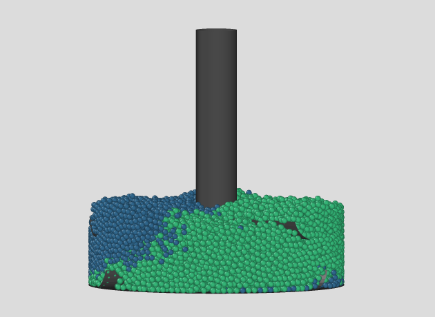
This GPU test case features a simple mixer configuration with one stationary blade set and another that rotates. Two particle types are introduced in separate inlet regions, and the heated mixer base warms the particles as they are blended throughout the process. The images show the state of the simulation at the last time step:

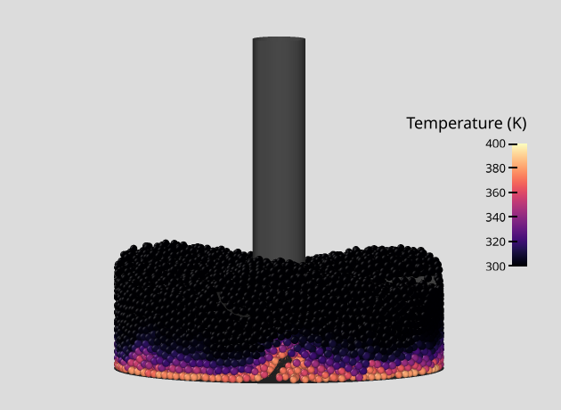
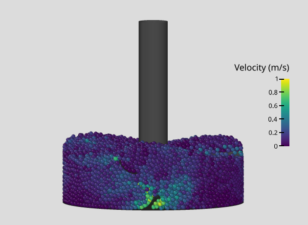
Name of the case: Project_Thermal_Mixer_GPU

Inserting & Mixing on the GPU

General settings

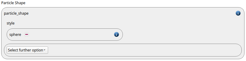
In this simulation we use particles of particle_shape type sphere:

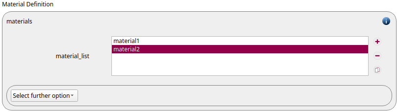
Two materials, material1 and material2, are defined:

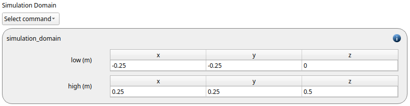
The simulation domain is defined with x and y dimensions ranging from -0.25 to 0.25 meters and the z dimension ranging from 0 to 0.5 meters:

Meshes and Regions

We start with defining the rotational motion for the mixing blades, using a mesh_module of type motion:

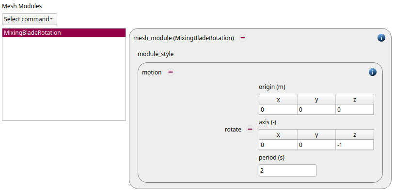
id	mesh_module | style | origin | axis | period
MixingBladeRotation	motion | rotate | ( 0, 0, 0) | ( 0, 0, -1 ) | 0.25

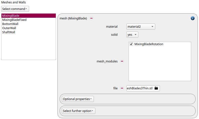
Then we insert the mesh for the blades that uses the just created mesh_module:

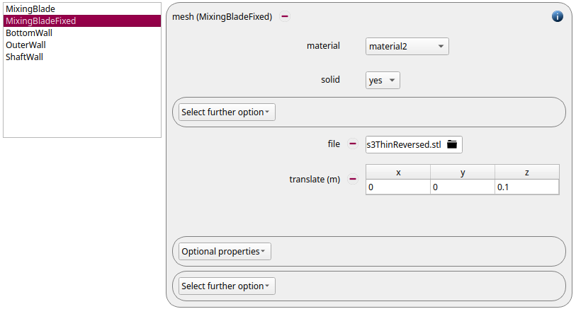
Next, the mesh for the fixed plates is inserted. This mesh is translated by 0.1 m in x-direction:

For the shaft of the mixer, the cylindric wall and the bottom three primitive walls are used:

id	type	center	normal	radius
BottomWall	disk	( 0, 0, 0.0 )	( 0, 0, 1 )	0.25
OuterWall	cylinder	( 0, 0, 0)	( 0, 0, 1 )	0.25
ShaftWall	cylinder	( 0, 0, 0)	( 0, 0, 1 )	0.04

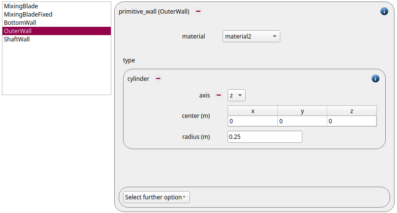
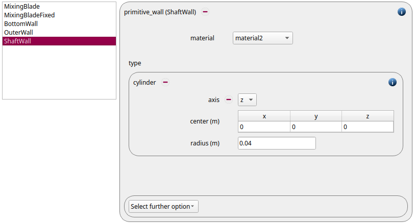
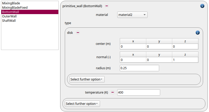
Please note that we assigned a temperature of 400K to the bottom plate.

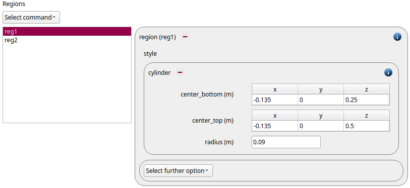
Finally we define two regions regions that we will be using for the insertion:

id	center_bottom	center_top	radius
reg1	( -0.135, 0, 0.25)	( -0.135, 0, 0.25)	0.1
reg2	( 0.135, 0, 0.25)	( 0.135, 0, 0.25)	0.1

Physics Models

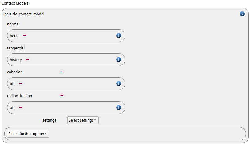
In the next step, the definition of the physics models takes place. For the particles we use the normal contact model hertz and the tangential model history.

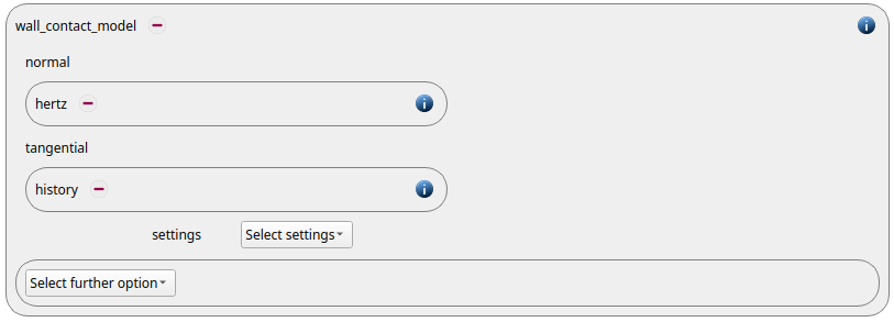
Since we added meshes and walls in the previous section a wall contact model was added automatically in this section. We use the same contact models as for the particles:

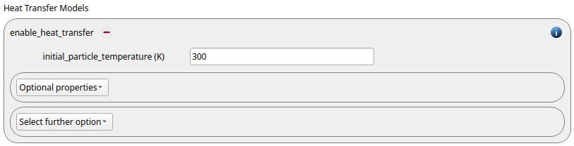
The calculation of the heat transfer is triggered by the enable_heat_transfer command command:

Finally also the gravity is defined:

Per default the gravity has a magnitude of 9.807 and acts into negative z-direction. These defaults can be changed by either setting the magnitude or the direction manually.

Particles

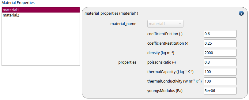
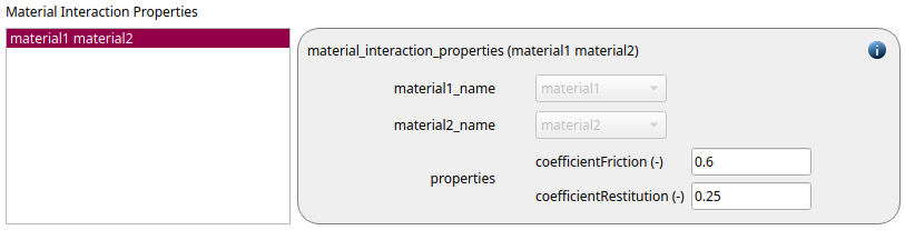
In the general settings tab we introduced two materials. Here we define the required material properties and material interaction properties.

	material1	material2
Density	2000	2000
Young’s modulus	5e6	5e6
Poisson ratio	0.3	0.3
Coefficient of restitution	0.25	0.25
Coefficient of friction	0.6	0.6
Thermal conductivity	100	100
Thermal capacity	100	100

	ParticleMaterial / WalllMaterial
Coefficient of restitution	0.25
Coefficient of friction	0.6

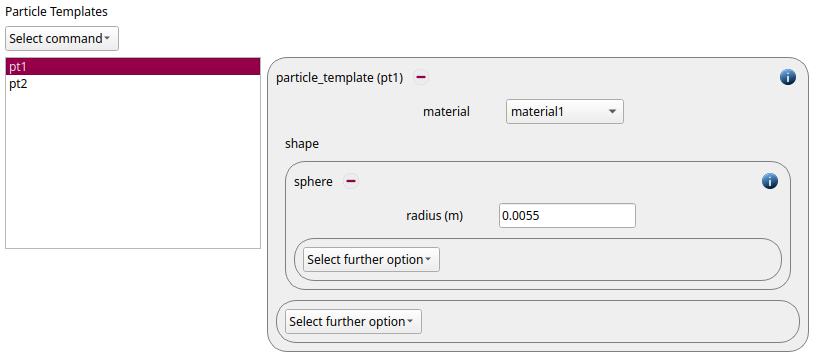
We now define two particle templates pt1 is of material1 and has a radius of 0.0055 m, pt2 is of material2 and has a radius of 0.006 m:

Then we define two particle distributions, one consists of pt1 and the other one of pt2:

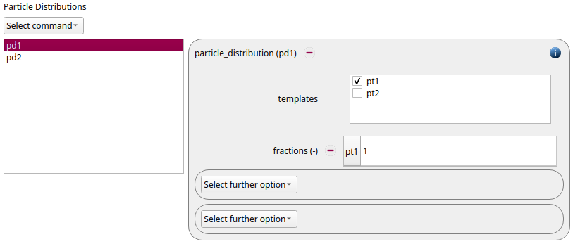
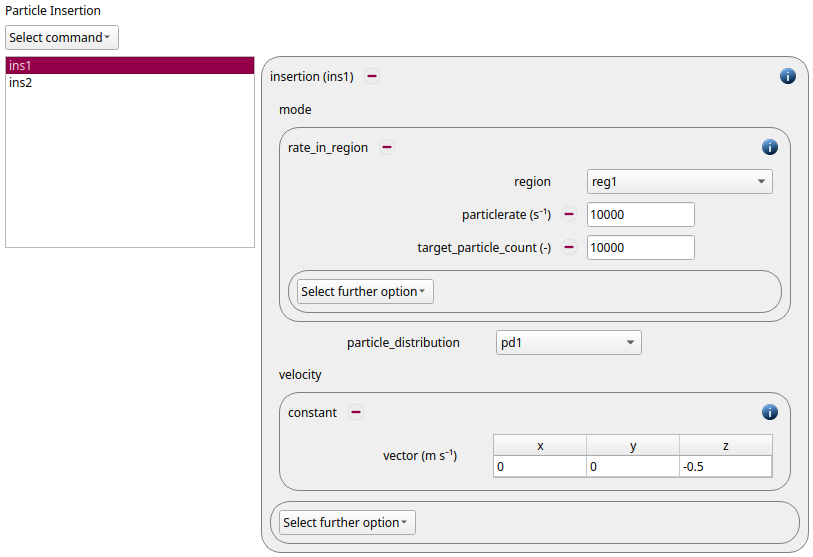
These two particle distributions are used for two insertion commands:

	ins1	ins2
region	reg1	reg2
particle_distriubtion	pd1	pd2
particlerate	10000	10000
target_particle_count	10000	10000
velocity vector	( 0, 0, -0.5)	( 0, 0, -0.5)

Simulation Control

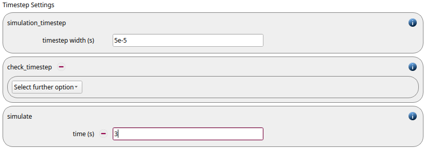
In this tab one first choses the time step settings such as the desired simulation timestep of 2e-5 seconds and the total simulation time of 3.0 seconds. Per default also the check_timestep command is enabled, which throws a warning when the time step exceeds 10 % of the Rayleigh or the Hertz timestep. These thresholds can be changed by setting an alternative value for hertz_fraction or rayleigh_fraction.

Output Settings

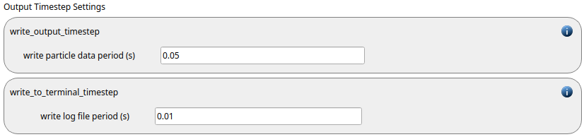
In this tab we first define the timestep width for the output to be 0.05 seconds and the terminal output to be 0.01 second:

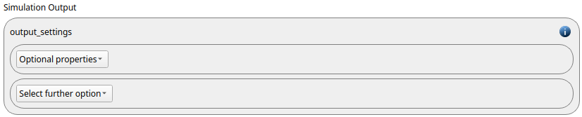
The output_settings command takes care that all particle information and the meshes are written to files accordingly. Furthermore it triggers the output of global quantities such as the kinetic energy of the particles or total normal and shear stresses onto meshes in the terminal. Please note that if the output of per-cell information on meshes such as velocity or stress are desired, the keyword mesh_properties has to be added and the required output has to be selected.

Running the Simulation

After saving the case we can change to the Simulation section. By hitting the Start button we can start running the GPU simulation. Have a look at the top of the log file for GPU architecture information:

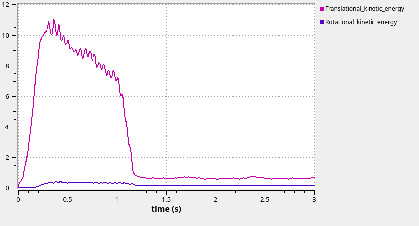
During the simulation, various quantities are displayed, such as the translational and rotational kinetic energy:

Postprocessing the Results

As soon as data was written to the post-folder within the simulation, it can be displayed with Ovito or Paraview. These images show the state of the simulation at the last timestep, the particles are colored accoding to velocity, temperature and radius respectively:

top