Simulation of a conveyor belt deformation using a coupled FEM-DEM simulation

In this tutorial we show how to set up a coupled FEM-DEM simulation using the GUI. The chosen finite element solver is Elmer (http://www.elmerfem.org/blog/)

Warning

Please note that this tutorial only works if you have an installation of Elmer on your machine! The GUI workflow can be used for setting up simulations on Windows, but running the simulation only works for Linux!

A step-by-step instruction of how to set up & run the simulation is shown in this screencast.

Elmer and ElmerGrid

The Elmer solver used in the coupled simulation is installed together with Aspherix. But in the preprocessing steps you will need ElmerGrid (https://www.nic.funet.fi/index/elmer/doc/ElmerGridManual.pdf), which is a mesh generation and manipulation utility.

To install Elmergrid you need a standalone Elmer installation. On Ubuntu/Debian you can use

sudo apt-add-repository ppa:elmer-csc-ubuntu/elmer-csc-ppa
sudo apt-get update
sudo apt-get install elmerfem-csc

Further information and instructions on how to install Elmer can be found here: https://www.csc.fi/web/elmer/binaries.

FEM Settings: Mesh and Boundary conditions

Before the we set up the DEM simulation we need to prepare the FEM simulation. Here we give a brief overview of the preprocessing step needed to set up the FEM part of the simulation. You will find the elmer_script.sif file in this tutorial folder, inside the data folder. A more detailed explanation, in particular on how to set up the ElmerSolver Input File (SIF) is given in the Aspherix solver FEM-DEM tutorial. Elmer will use the plain text file named ELMERSOLVER_STARTINFO to locate the sif file. ELMERSOLVER_STARTINFO must be located in the same folder where the simulation is run, and have to contain the location of the sif file. In this case, data/elmer_script.sif.

Warning

The ELMERSOLVER_STARTINFO is not automatically created/copied by the GUI and has to be created/copied manually by the user.

Mesh preparation

In the tutorial folder, you will find the conveyor belt mesh file (meshes.unv). In order to be read by Elmer the unv file has to be converted into the ElmerSolver format. This can be done with the command:

ElmerGrid 8 2 meshes.unv -autoclean

This command generates the folder meshes, which contains a series of files with all the mesh information needed by Elmer.

Boundary conditions

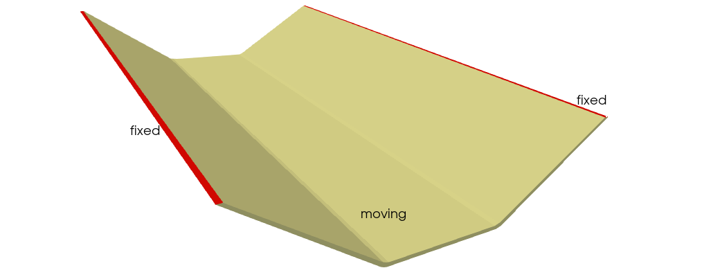
The boundary conditions are defined in the elmer_script.sif file. In this case, as shown in the figure, there are two boundary condition for the FEM simulation. We have the fixed boundary, shown in red, where we impose zero displacement.

Boundary Condition 1
   Target Boundaries(1) = 2
   Name = "fixed"
   Displacement 3 = 0
   Displacement 1 = 0
   Displacement 2 = 0
End

We have the moving boundary, shown in yellow, where the simulation exchanges the stresses between FEM and DEM.

Boundary Condition 2
   Target Boundaries(1) = 1
   Name = "moving"
   Force 1 = Variable Coordinate
      Procedure "Aspherix_FEM_coupling" "mesh_force_x"
   Force 2 = Variable Coordinate
      Procedure "Aspherix_FEM_coupling" "mesh_force_y"
   Force 3 = Variable Coordinate
      Procedure "Aspherix_FEM_coupling" "mesh_force_z"
End

DEM Settings

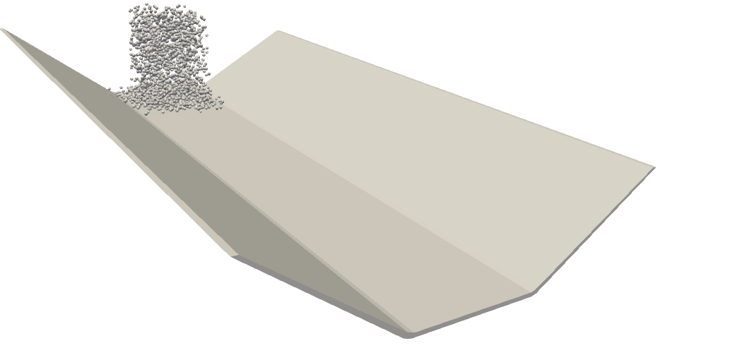
This is the setup for the DEM part of the simulation. We continuously insert particles in an insertion region above the conveyor belt. The particles hit the belt and are transported along by a surface velocity. The impact of the particles on the mesh induces a deformation, computed by the FEM solver.

General settings

We start with setting the particle_shape command type to sphere:

We keep the default material material1:

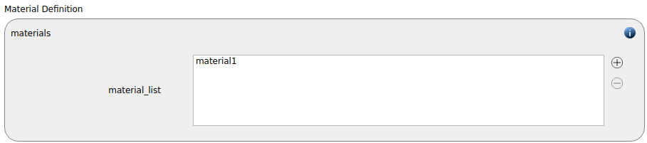
Remark: Please avoid too long material names as this could lead to issues later on (ideally less than 12 characters).

The simulation_domain command with x dimensions ranging from -0.5 to 0.5 m, y dimensions ranging from -2 to 0.2 m and z dimensions ranging from -0.5 to 0.3 m is created:

FEM coupling (in CFD tab)

In order to have a coupled simulation, Aspherix requires the enable_fem_coupling command command. This command can be added in the “CFD” tab:

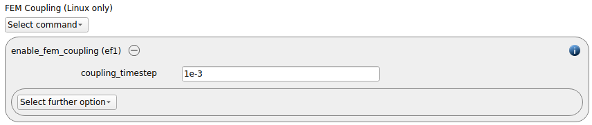
It is important to add this command before creating those mesh commands that refer to meshes that are also considered in Elmer, since they require a reference to the ID of the coupling command.

Meshes and regions

We return to the Meshes and Regions tab, where the meshes can be defined. The stresses sent from the DEM simulation to the FEM simulation need to be averaged over time to capture the correct behaviour. Therefore, we need the mesh_module stress_average to be activated:

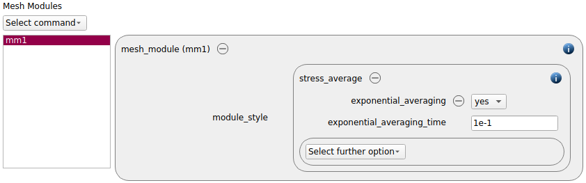
The meshes can then be added. We add a fixed and a moving mesh command. Please note the mesh_module added to the moving mesh.

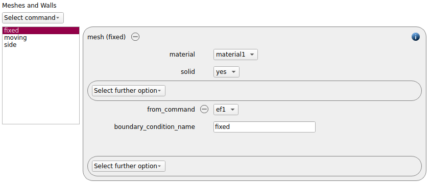
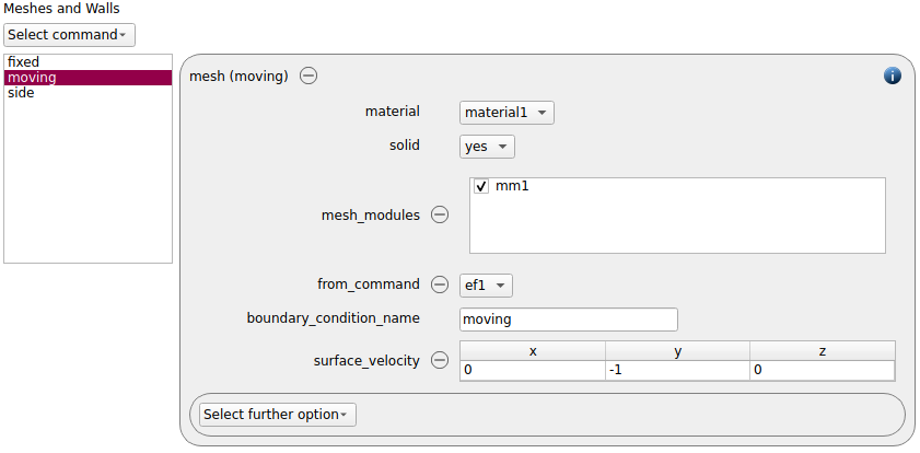
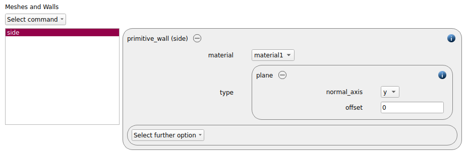
We also define a primitive wall normal to the y axis with a 0 offset.

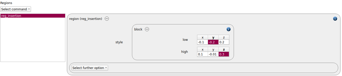
We proceed by defining a region command above the conveyor belt for particle insertion:

Physics models

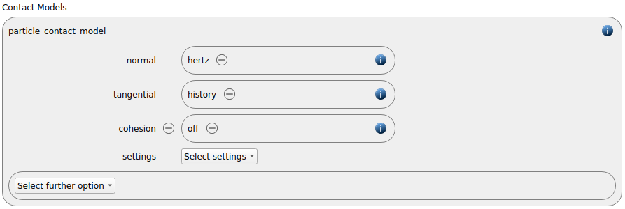
As particle contact model we use normal hertz and tangential history:

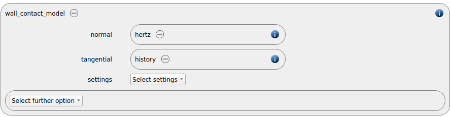
The same settings are chosen for the wall contact model:

We keep the default setting for gravity:

Particles

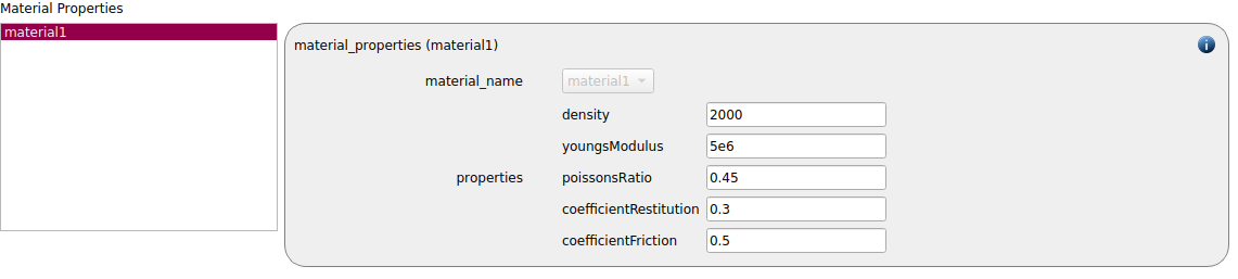
In the particles tab we complete the material definition by setting the material properties. The material density is set to 25 kg/m3, the Youngs Modulus 5e6 Pa, the Poissons ratio is 0.3, the coefficient of restitution is 0.5 and the coefficient of friction is 0.5:

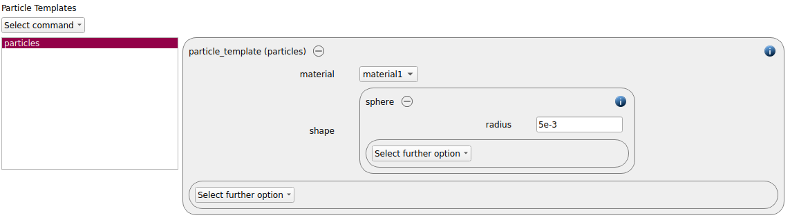
A particle templates with a 5 mm radius is generated:

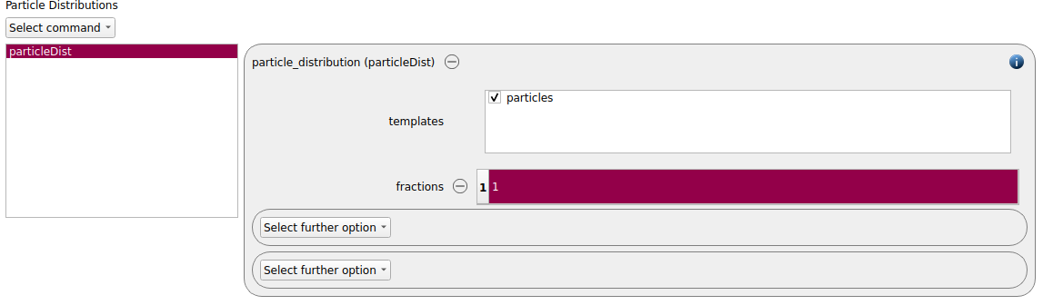
The template is used to create a particle distribution:

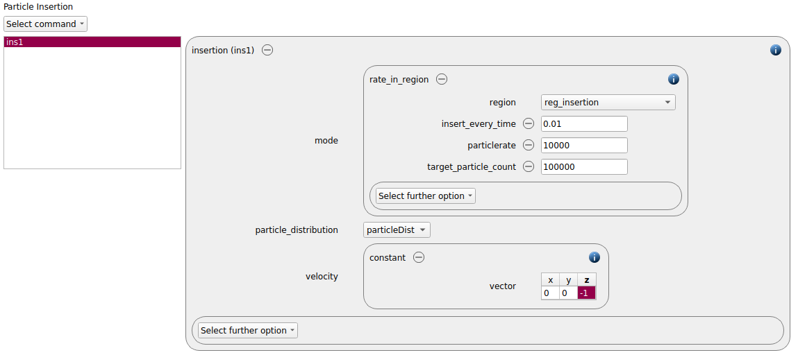
An insertion command command of type rate_in_region is used for particle generation, with the following set-up:

Simulation control

In this tab, we define time-step settings such as the desired simulation timestep of 1e-5 seconds and the total simulation time of 10.0 seconds. Per default also the check_timestep command command is enabled, which throws a warning when the time step exceeds 10 % of the Rayleigh or the Hertz timestep. These thresholds can be changed by setting an alternative value for hertz_fraction or rayleigh_fraction.

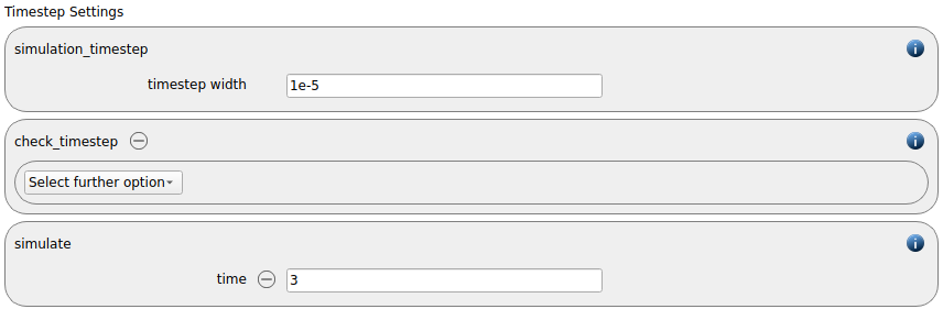
The enable loadbalancing command is added automatically. When running simulations in parallel, it ensures an optimal distribution of the load on the processors.

Output control

In this tab we first define the timestep width for the file and the terminal output:

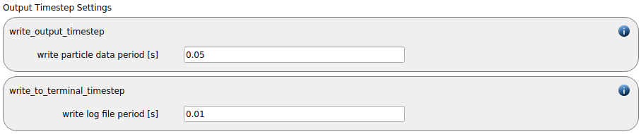
The output_settings command takes care that all particle and meshes information is written to files accordingly. Furthermore, it triggers the output of global quantities such as the kinetic energy of the particles or total normal and shear stresses onto meshes in the terminal.

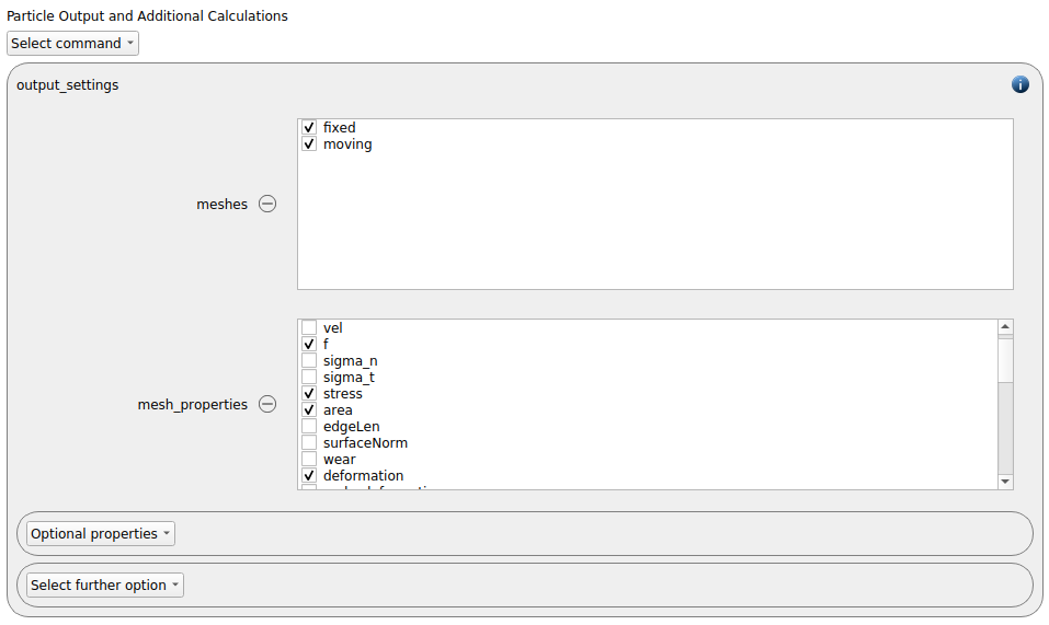
Remark: please note that per default all meshes are written by the output settings, but without potentially available values for stress, wear, velocity etc. Please use the mesh_properties command for producing the desired output.

The setup of this case is complete now, we can save the setup and move on to the simulate section.

Running the simulation

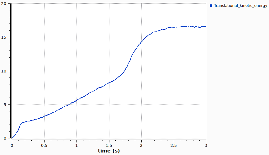
The simulation can be started now, the graphs below show the number of particles during the simulation we well as the total kinetic energy:

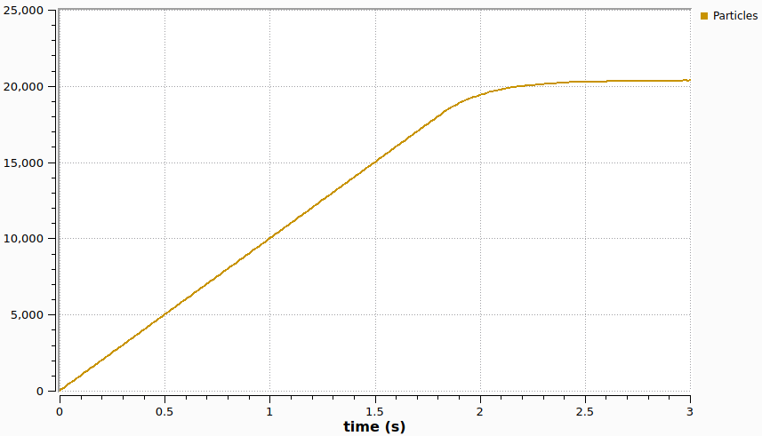
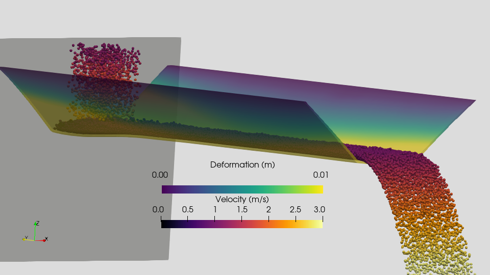
The result can be visualized in Paraview: