 Home
HomeDrag modelling with DEM and CFD-DEM
In this tutorial we show different possibilities of drag modelling for particle simulations.
The goal is to model particles that fall a stream of particles that falls onto a chute and is exerted to a crossflow underneath the chute:
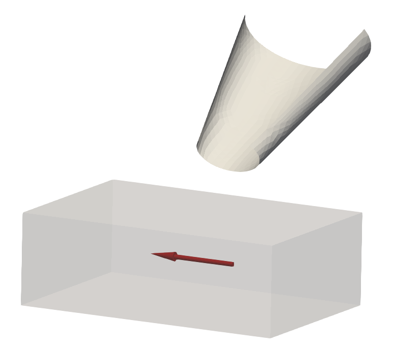
For drag modelling we require information about the fluid that exerts the drag (density, viscosity, velocity). We start with setting up a basic DEM case, where particles fall onto a transport chute (no drag). In the first step we define uniform velocities in different regions, in the second step we use a fluid velocity field obtained by a CFD simulation. Then, we use a sequence of fluid fields. This already ressembles a simple two-way coupling approach, where the particles see different fluid fields at different time steps, only the fluid field is not influenced by the particles’ presence. Finally we conclude with two fully four-way coupled simulations, in one case the drag force is calculated on the CFD side and in the other case the drag force is calculated directly on the DEM side.
The results we obtain in this case differ a fair bit, which shows that the choice of the drag modelling method is crucial for obtaining accurate results efficiently. Please note that the presented case (very low particle density in comparison to the surrounding fluid, relatively densly packed particles at least in certain areas) is not a standard application for one-way coupling (no matter if basic or transient) and it is expected that the results match for the different methods. We have picked this setup to exaggerate the influence of the different approaches.
Warning
Please note that this tutorial only works if you have an installation of CFDEMcoupling on your machine! The GUI workflow can be used for setting up simulations on Windows, but running the simulation in the explained way only works for Linux!
A step-by-step instruction of how to set up & run the simulation is shown in this <https://vimeo.com/713164906> screencast.
Base case
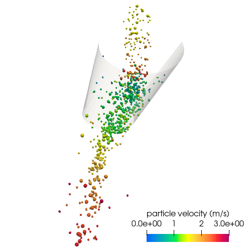
This is the basic setup for the DEM part of the simulation. We continuously insert particles in an insertion region above the chute. The particles hit the chute and slide down. In the basic case the particle stream that forms at the end of the chute does not see any forces from a surrounding fluid.
General settings
We start with setting the particle_shape command type to sphere:

We keep the default material material1:
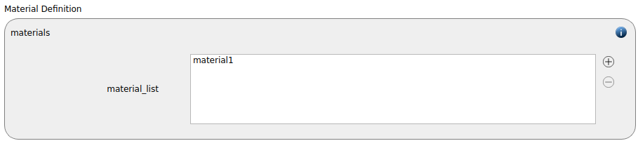
Remark: Please avoid too long material names as this could lead to issues later on (ideally less than 12 characters).
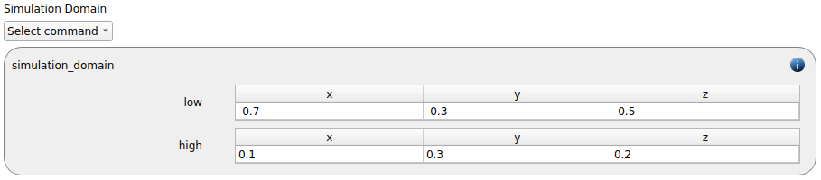
The simulation_domain command with x dimensions ranging from -0.7 to 0.1 m, y dimensions ranging from -0.3 to 0.3 m and z dimensions ranging from -0.5 to 0.2 m is created:
Meshes and regions
In the meshes and regions tab we start with defining the mesh of the chute:
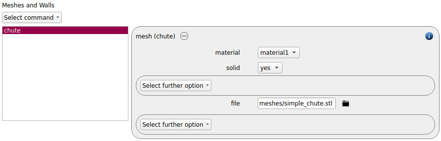
Since the chute will be used as wall, we keep the option “solid yes”.
For the particle insertion later on we define a cylindric region above the chute:
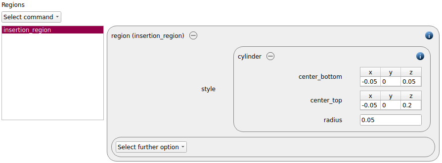
The center of the cylinder has and x-position of -0.05 m, a y-position of 0 and spans between 0.05 and 0.2 m in z-direction. The radius of the cylinder is 0.05 m.
Physics models
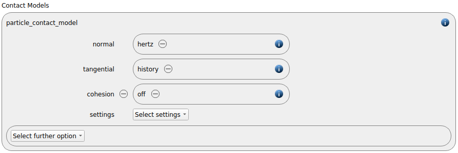
As particle contact model we use normal hertz and tangential history:
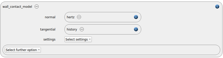
The same settings are chosen for the wall contact model:
We keep the default setting for gravity:

Particles
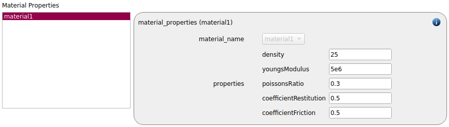
In the particles tab we complete the material definition by setting the material properties. The material density is set to 25 kg/m3, the Youngs Modulus 5e6 Pa, the Poissons ratio is 0.3, the coefficient of restitution is 0.5 and the coefficient of friction is 0.5:
Two particle templates with particles of 3 and 5 mm radius are generated:
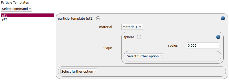
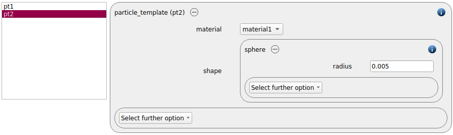
The two templates are used to create a particle distribution that consists of 50% smaller particles and 50% bigger particles:
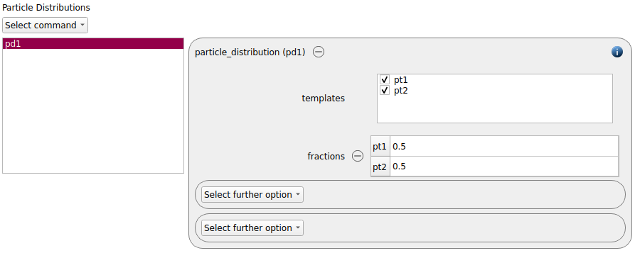
Per default, the particle distribution is mass-based, but by using the keyword mode this can be changed to number-based.
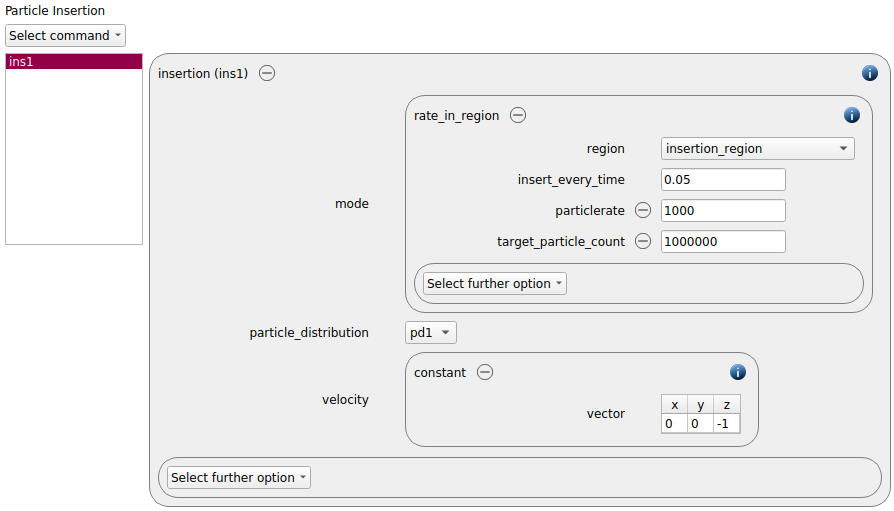
An insertion command command of type rate_in_region is used for particle generation:
Simulation control
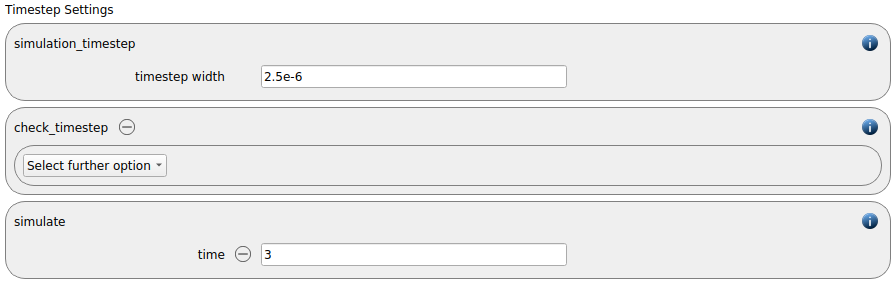
In this tab one first choses the time step settings such as the desired simulation timestep of 2.5e-6 seconds and the total simulation time of 3.0 seconds. Per default also the check_timestep command command is enabled, which throws a warning when the time step exceeds 10 % of the Rayleigh or the Hertz timestep. These thresholds can be changed by setting an alternative value for hertz_fraction or rayleigh_fraction.
The enable loadbalancing command is added automatically. When running simulations in parallel, it ensures an optimal distribution of the load on the processors.

Output control
In this tab we first define the timestep width for the file and the terminal output:
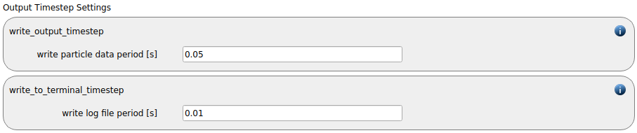
The “output_settings” command the takes care that all particle information and the meshes are written to files accordingly. Furthermore it triggers the output of global quantities such as the kinetic energy of the particles or total normal and shear stresses onto meshes in the terminal.
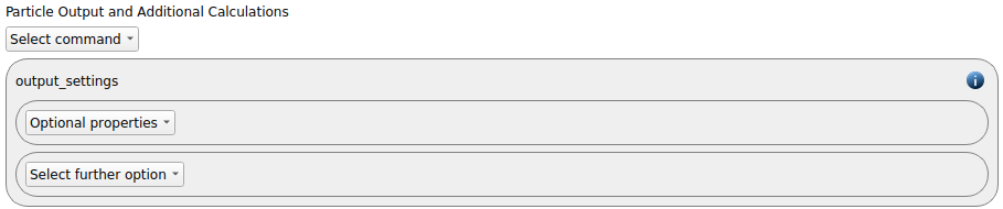
Remark: please note that per default all meshes are written by the output settings, but without potentially available values for stress, wear, velocity etc. Please use the mesh_properties command for producing the desired output.
The setup of this case is complete now, we can save the setup and move on to the simulate section.
Running the simulation
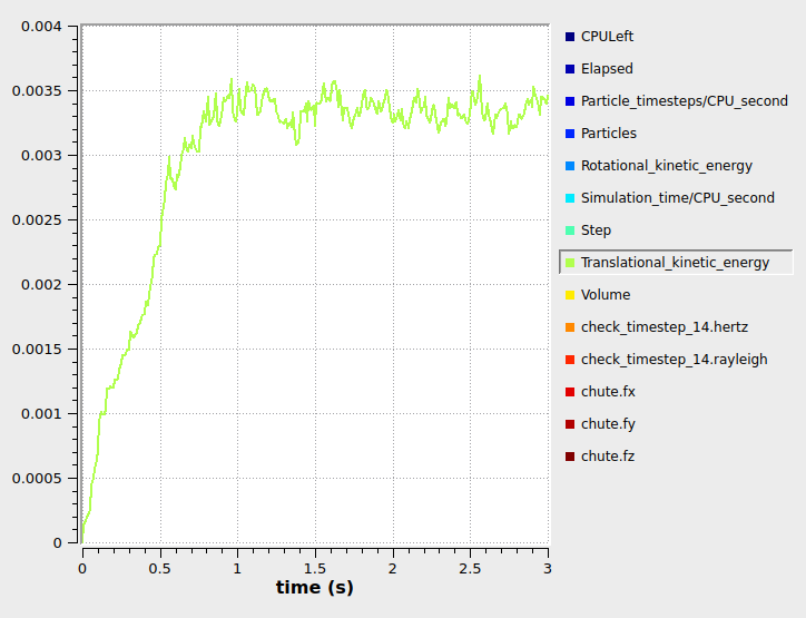
The simulation can be started now, the graphs below show the number of particles during the simulation we well as the total kinetic energy:
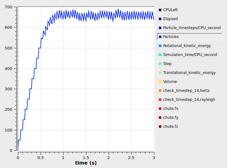
The result can be visualized in Paraview:
One-way coupling - constant velocity
We clone the “Base case” and convert it to a one-way coupled simulation now. For applying different fluid velocities in two different regions (cross flow region and “everywhere else”) we go to the meshes and regions tab to define the regions first:
Meshes and regions
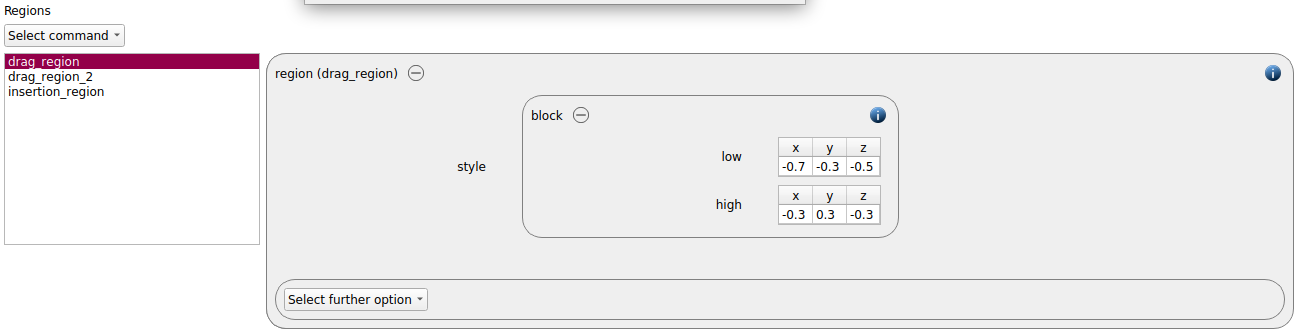
The crossflow region (here we call it region_drag) is a region of type box that reaches from -0.7 to -0.3 in x-direction, from -0.3 to 0.3 in y-direction and from -0.5 to -0.3 in z-direction:
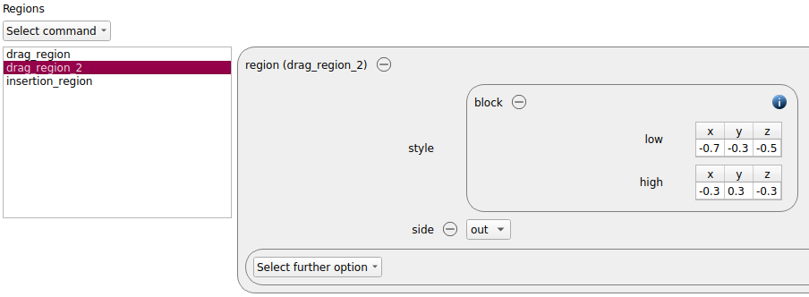
For obtaining a region that consists of anything but the drag_region we define a box with the same dimensions and the additional keyword “side out”:
Coupled Simulation
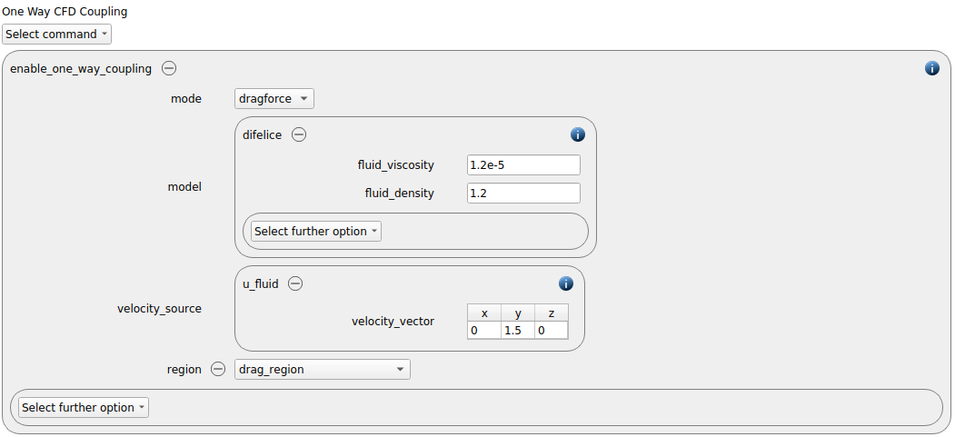
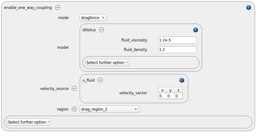
Now, we apply two enable_cfd_coupling command commands, one with U_fluid (0,1.5,0) and one with U_fluid (0,0,0). In both cases we use a fluid viscosity of 1.2e-5 and a fluid density of 1.2:
Running the simulation
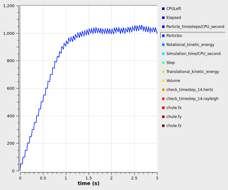
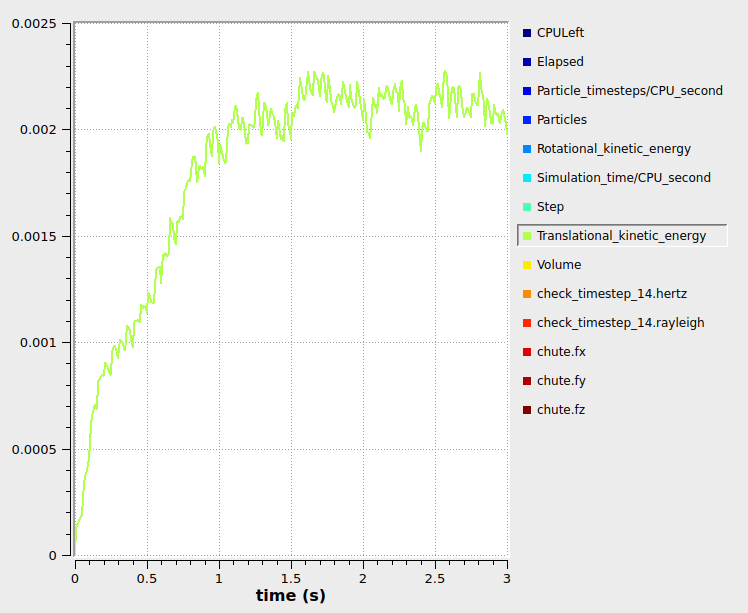
We launch the simulation on 2 cores and get the following output for particle number and kinetic energy:
When postprocessing the result in Paraview the differences to the base case become evident:
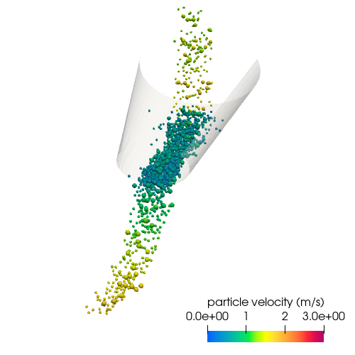
Due to the drag force we can see that more particles are accumulated at the chute, and the particle stream below the chute is deviated in the direction of the fluid flow. Please note that in this and the following two cases the particle velocity has no impact on the fluid field.
One-way coupling - velocity field
Again, we start with cloning the base case. In this setup we are using a single enable_one_way_coupling command that has a complete fluid field as input. It is therefor not required to define any regions. The fluid field was generated by a CFD calculation that can be found in the project repo (CFD.zip). For preparing the case, please use the provided Allrun.sh script, for running the simulation please use “pisoFoam”. The data can be extracted from within Paraview (using the Save Data functionality and making sure that only the U point data is written). The generated file, however, requires some postprocessing - the comma delimiters must be replaced by spaces, and the header must look as follwing:
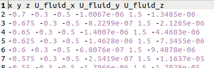
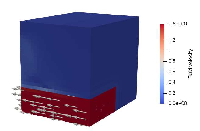
As velocity field we are using the velocities from the last simulation time step:
Note
A copy of the velocity field can be found in the installation folder (default: DCS-Computing/Aspherix-…/examples/gui/CFDEM_Project_Chute/one_way_coupling_field/data/vel_29.csv). A fully prepared CFD case can be found in the examples folder of the installation (default: DCS-Computing/Aspherix-…/examples/gui/CFDEM_Project_Chute/CFD.zip).
Coupled Simulation
When using enable_one_way_coupling for the option U_fluid_file, you are required to define a bin size, which is set to 0.02 in this case:
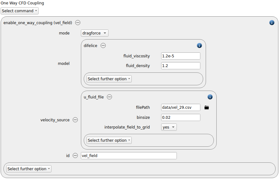
The bin size is the cell size of the regular grid that is formed in the background. Please note that interpolate_field_to_grid should always be set to yes, otherwise the provided velocity field must match the field that Aspherix generates internally.
Running the simulation
After adding this setting and saving the simulation can be launched, the below graphs show the number of particles and the kinetic energy:
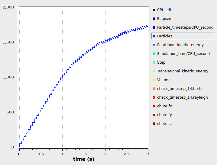
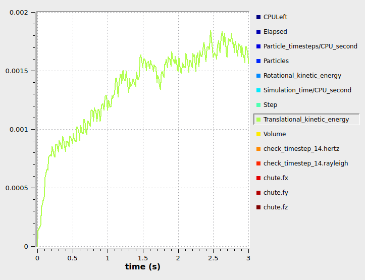
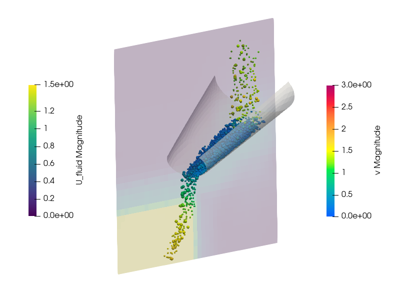
In Paraview, we can postprocess the DEM results as usual, by auto loading them through the “Start Paraview” button. The velocity field data can be imported separately (use the File/Open in Paraview). For assigning a matching time step to the velocity fields, please use the “Temporal Shift Scale” filter with a scale factor that matches the time step of the DEM output timestep (0.05 in this case).
Transient one-way coupling
Again, we start by cloning the base case. In transient one-way coupled simulations we use a series of velocity fields (e.g., obtained from a stand-alone CFD simulation) as input. The base for the velocity field data is the same CFD case as above, but in this case we use every other data field (so 30 in total for 3 seconds of simulation time).
Note
The velocity field sequence file and all velocity fields can be found in the examples folder of the installation (default: DCS-Computing/Aspherix-…/examples/gui/CFDEM_Project_Chute/one_way_coupling_transient/data/vel_29.csv).
Coupled simulation
For transient one way coupling we use the enable_one_way_coupling command with the option U_fluid_sequence_file:
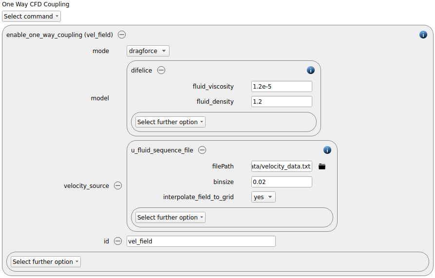
The sequence file contains a a list of all velocity files that are use as input together with the time step at which they were taken:
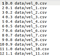
Each individual velocity file must be of the same format at shown in the previous section.
Running the simulation
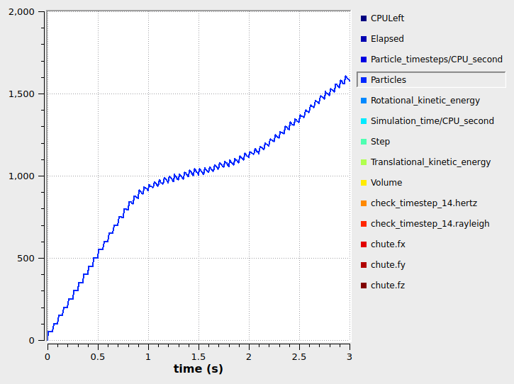
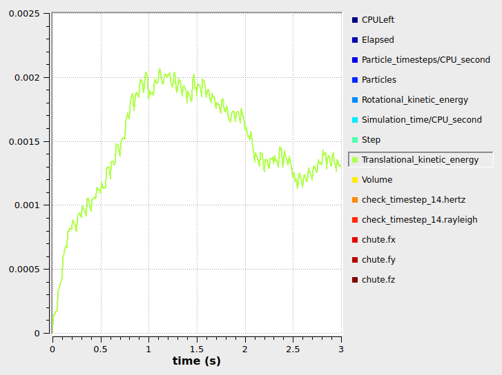
After adding this setting and saving the simulation can be launched, the below graphs show the number of particles and the kinetic energy:
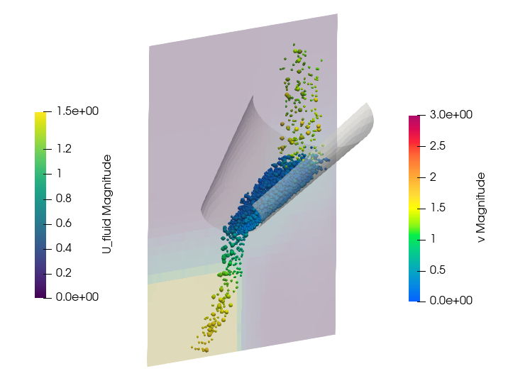
In Paraview, we can postprocess the DEM results as usual, by auto loading them through the “Start Paraview” button. The velocity field data can be imported separately (use the File/Open in Paraview). For assigning a matching time step to the velocity fields, please use the “Temporal Shift Scale” filter with a scale factor that matches the time step of the DEM output timestep (0.05 in this case).
In all cases discussed so far the particles had no influence on the fluid field. For dilute particle regimes this might be suitable, but in other cases one might want to run fully four-way coupled cases. In the following we show how to create fully coupled cases on the basis of a pure DEM and a pure CFD case.
Full CFD-DEM coupling (DEM drag)
Again, we start by cloning the base case. This time, the goal is to calculate the drag forces on the DEM side, based on fluid information that is obtained by the CFD calculation. The CFD on the other hand sees that particles and accounts for their presence.
Note
A fully prepared coupled case can be found in the examples folder of the installation (default: DCS-Computing/Aspherix-…/examples/gui/CFDEM_Project_Chute/CFD_DEM_drag.zip).
Coupled simulation
With the enable_dem_drag command command we indicate that the drag force calculation is carried out on the DEM side:
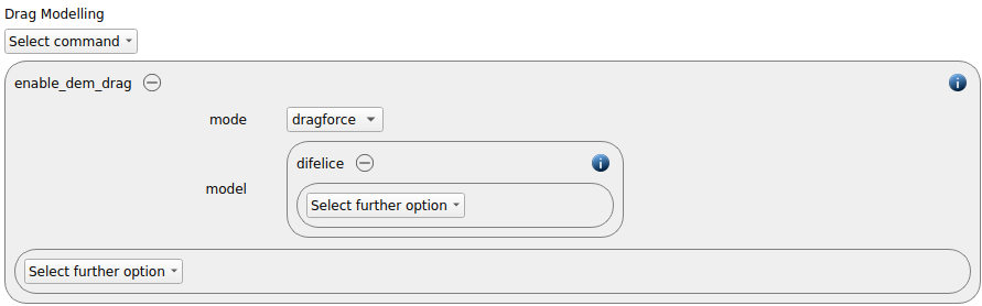
We are selecting the DiFelice drag model. The enable_cfd_coupling command command is used to establish the four-way coupling on the DEM side:

Information about fluid density, viscosity and velocity is provided by the CFD calculation.
On the DEM side these are all settings required, the next step now consists in preparing the pure CFD case for a coupled calculation. We therefore make a copy of the folder CFD (e.g., CFD_DEM_drag) and move to the CFD-DEM Setup tab:
CFD-DEM Setup tab
There, we start filling the form. We select the input script of the current case as “Path to DEM input script” and set the correct path to the CFD case directory. We use particle shape sphere, and the fluid density is set to 1.2 (just as in the DEM cases previously). The solver we are using is cfdemSolverPiso and the model type for the equations is B. Please note that DEM based drag calculations are only possible with model type B. The drag force will not be scaled additionally, the standard locate model engine is used and we will run the simulation on 2 processors. We use the simple case decomposition scheme to decompose the mesh in 2 partitions in x direction, whereas y and z remain undivided.
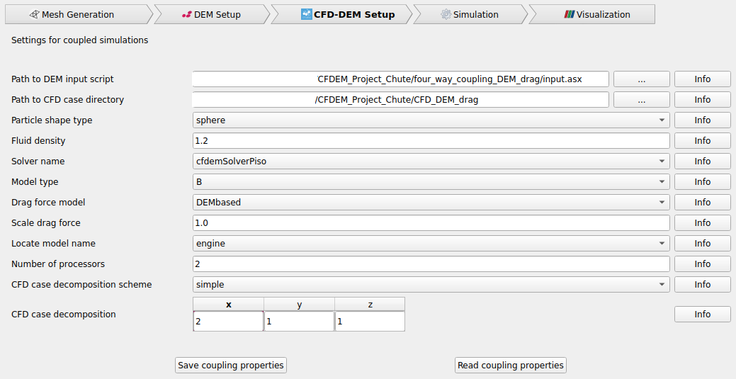
By pressing the “Save coupling properties” button the CFD case is now converted to a coupled CFD-DEM case. Missing files are copied to the according locations.
Please note that the CFD-DEM Setup tab is a tool that helps to generated coupled setups, but that does not establish a lasting connection between the active DEM case and the selected CFD folder. When re-opening the simulation project, you will not automatically find all settings auto-filled in the form. For checking the settings of a case you can use the “Read coupling properties” button.
Running the case
Before running the simulation please open a terminal and navigate to the CFD_DEM_drag folder. Execute decomposePar to prepare the case for a parallel run. Now the coupled simulation can be started.
There are two possibilities to launch the simulation:
1) Split run: Aspherix and the CFDEMcoupling solver can be launched in a side-by-side mode. Please open the project in the GUI and move to the Simulation tab of the DEM_run case. At the same time open a terminal and navigate to the CFD folder (must either be converted to the coupled folder by yourself or the unzipped CFD_coupled.zip folder that was renamed to CFD). Then prepare the CFD simulation (run blockMesh & decomposePar). Then type “mpirun -np 4 cfdemSolverPiso -parallel” in the terminal and hit enter. Without loosing much time click the “Run simulation” button in the GUI. The global DEM output is visulized in the GUI while the simulation is running.
2) Combined run command: the “cfdemSimulate” command can be used to launch a coupled simulation directly within the terminal and with a single command. It does not require a separate simulation launch of the DEM part of the case within the GUI. When launching the simulation this way the global DEM output in the GUI is not updated. The command requires information about the used solver, the DEM input script and the number of processors used in the simulation:
cfdemSimulate -in ../four_way_coupling_DEM_drag/input.asx -solver cfdemSolverPiso -np 2
Please type “cfdemSimulate –help” to check the options for this command.
If you selected possibility 1 then the number of particles and the kinetic energy are displayed in the Simulation tab of the GUI:
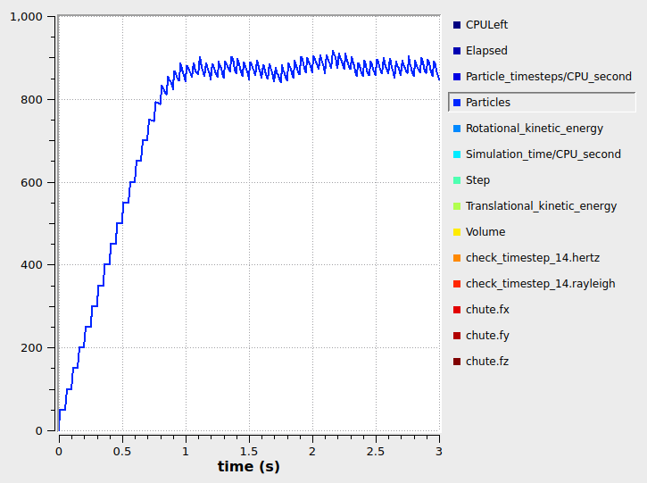
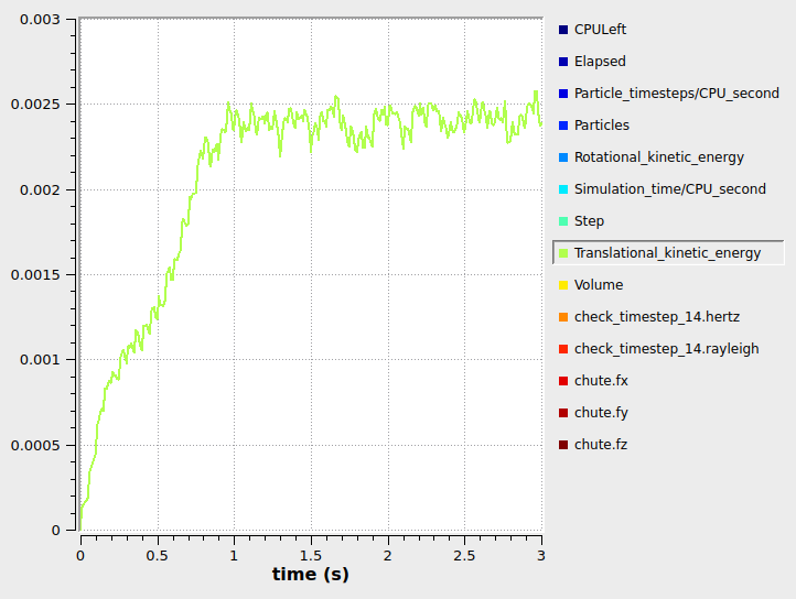
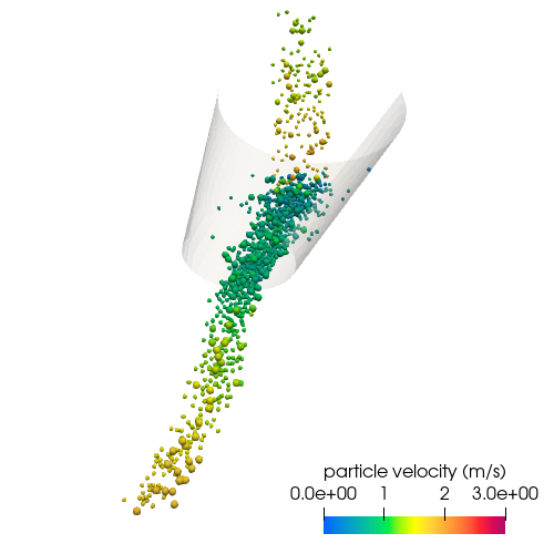
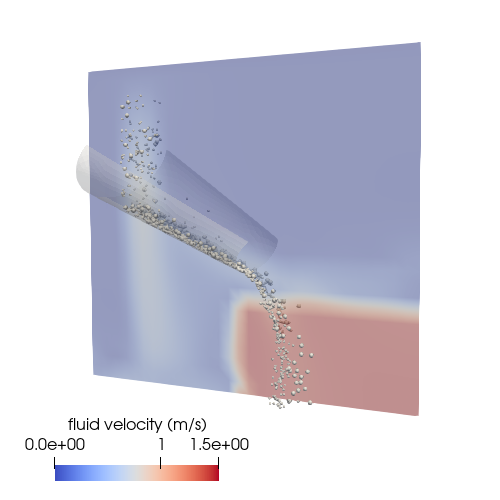
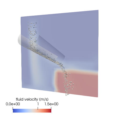
The DEM part of the result can be loaded in Paraview as usual, the CFD part of the data can be postprocessed with the CFDEMcoupling Paraview macro. Please make sure that the case type of the CFD data is set to “Decomposed case” before applying the macro:
Full CFD-DEM coupling (CFD drag)
Again, we start by cloning the base case. This time, the goal is to calculate the drag forces on the CFD side. Again, the CFD sees the particles and accounts for their presence.
Note
A fully prepared coupled case can be found in the examples folder of the installation (default: DCS-Computing/Aspherix-…/examples/gui/CFDEM_Project_Chute/CFD_CFD_drag.zip).
Coupled simulation
In this case, we only require the enable_cfd_coupling command:

With this step, all required changes on the DEM side are completed. We make another copy of the CFD folder and call it CFD_CFD_drag. The navigate to the CFD-DEM Setup tab.
CFD-DEM Setup tab
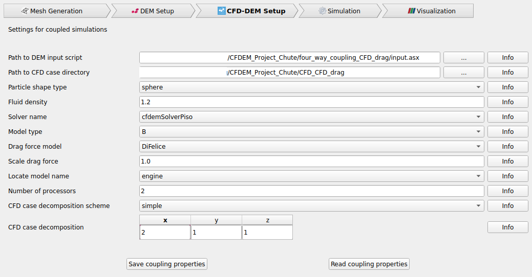
Most settings in this tab is similar, the main difference are the different pathes for input script and CFD folder as well as the drag model that is now set to DiFelice:
Running the simulation
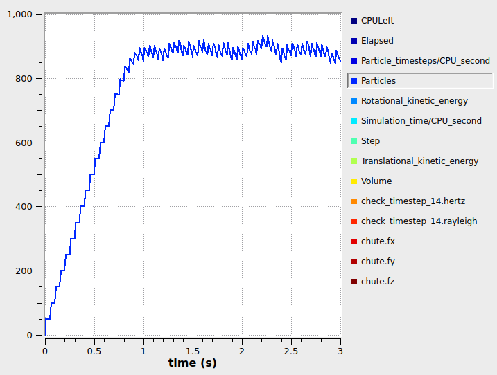
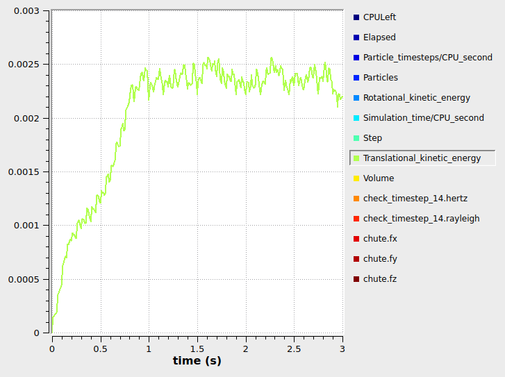
For running the case we have the same options as for the previous one. The particles and kinetic energy can be visualized in the GUI if the “split run” (possibility 1) is chosen:
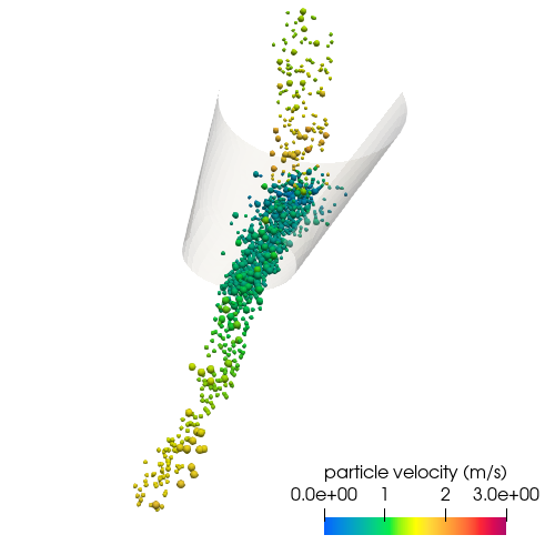
Also postprocessing in Paraview works analogously:
Name of the case: CFDEM_Project_Chute