 Home
HomeRotating Drum (GPU)
This tutorial is only available for Linux.
This GPU tutorial of a rotating drum consists of two simulations: first, particles are inserted with a single pack insertion and allowed to settle. Then, shearforces are applied to the walls to mimique a rotational motion of the primitive-wall cylinders.
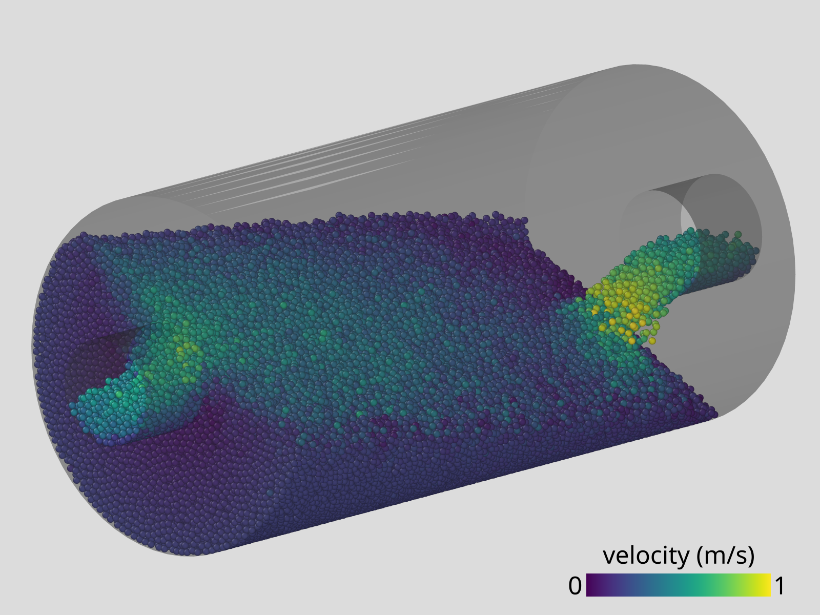
Name of the case: Project_Rotating_Drum_GPU
Inserting & Rotation on the GPU
General settings
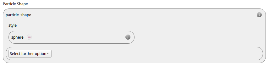
In this simulation we use particles of particle_shape type sphere:
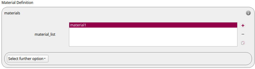
The single material is defined for both particles and walls:
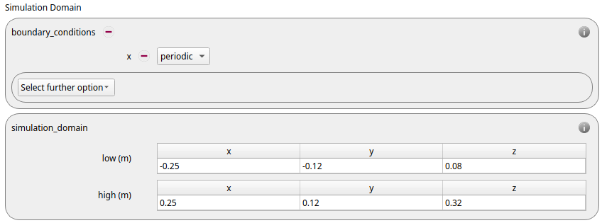
The simulation domain is defined with the x dimension ranging from -0.25 to 0.25 meters, the y dimension ranging from -0.12 to 0.12 meters, and the z dimension ranging from 0.08 to 0.32 meters. Periodic boundaries are set in the x dimension to recirculate the particle flow.
Meshes and Regions
In this setup we use primitive walls for the drum, all components are of type material1.
We create the cylindrical walls using primitive walls of type cylinder.
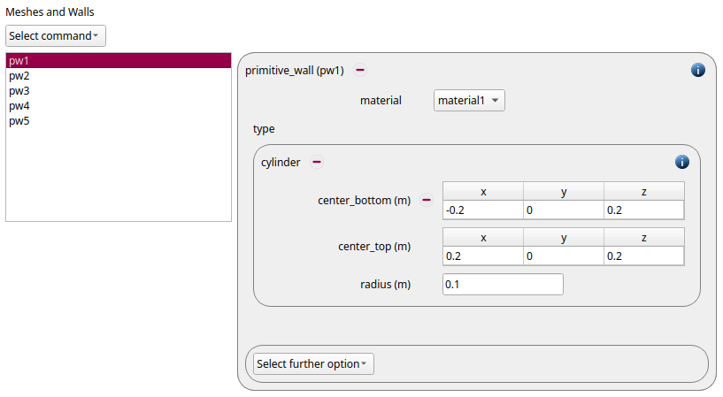
id |
type |
center_bottom |
center_top |
radius |
|
|
( -0.20, 0.0, 0.2) |
( 0.20, 0.0, 0.2) |
0.20 |
|
|
( -0.25, 0.0, 0.2) |
(-0.20, 0.0, 0.2) |
0.03 |
|
|
( 0.20, 0.0, 0.2) |
( 0.25, 0.0, 0.2) |
0.03 |
We create annulus caps for the main cylinder using
primitive walls of type disk (using an inner_radius
to cut out a hole):
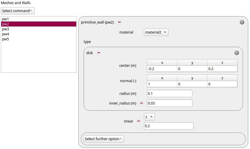
id |
type |
center |
normal |
radius |
inner_radius |
|
|
( -0.20, 0.0, 0.2) |
( 1, 0, 0 ) |
0.20 |
0.03 |
|
|
( 0.20, 0.0, 0.2) |
( 1, 0, 0 ) |
0.20 |
0.03 |
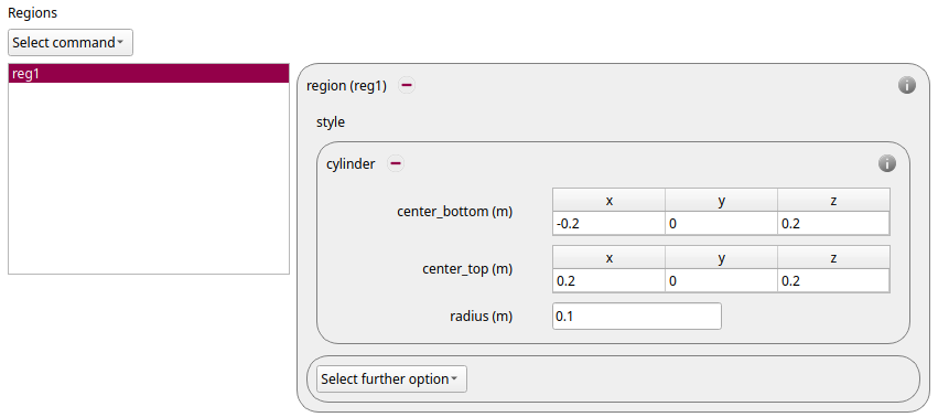
Finally, we define the region of shape cylinder that
we will be using for the insertion.
id |
center_bottom |
center_top |
radius |
|
( -0.20, 0, 0.20) |
( -0.20, 0, 0.20) | 0.1 |
|
Physics Models
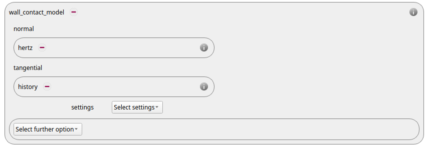
In the next step, the definition of the physics models takes place. For the particles we use the normal contact model hertz and the tangential model history.
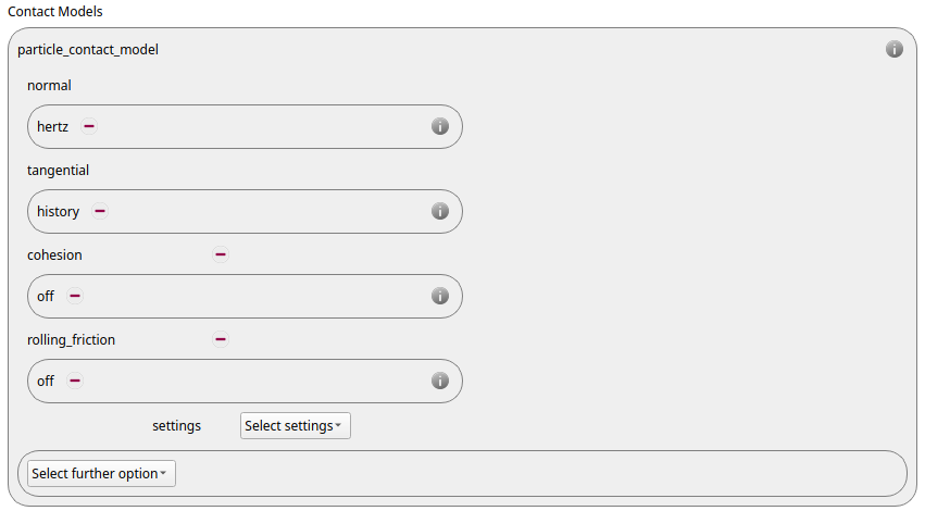
Since we added meshes and walls in the previous section a wall contact model was added automatically in this section. We use the same contact models as for the particles:
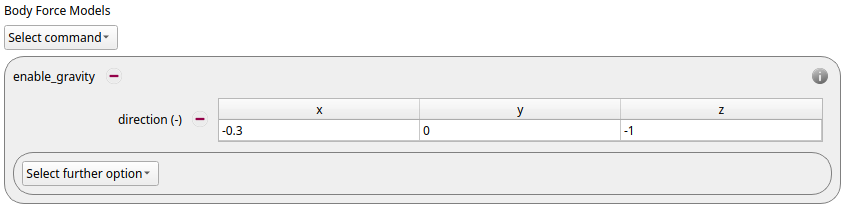
Finally, a gravity body force is defined. We define the direction of the gravity force to be primarily downwards (-z) but also slightly slanted to the left (-x) Per default the gravity has a magnitude of 9.807.
Particles
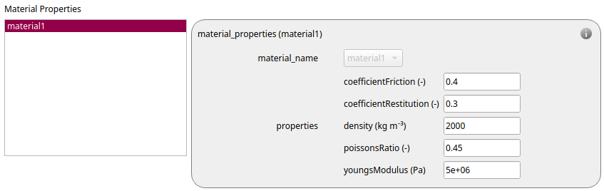
In the general settings tab we introduced our material material1, and now we define the required
material properties for that material:
|
|
Density |
2000 |
Young’s modulus |
5e6 |
Poisson ratio |
0.45 |
Coefficient of restitution |
0.4 |
Coefficient of friction |
0.3 |
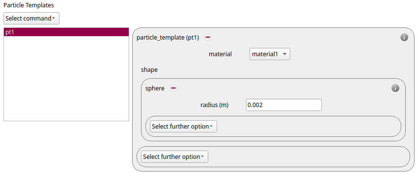
We now define a particle template named pt1 of
shape sphere where we set the particle radius (and also set the material):
Then we define a particle distribution named
pd1 using the abovementioned particle template.
Since we have only 1 particle template it composes 100% of the distribution.
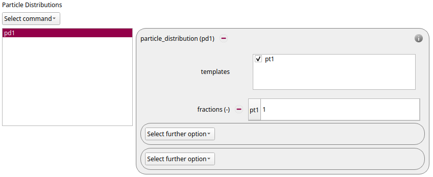
Finally, we can define our insertions named ins1
using our particle distribution pd1.
We use a single pack insertion to add 100000 particles into the domain.
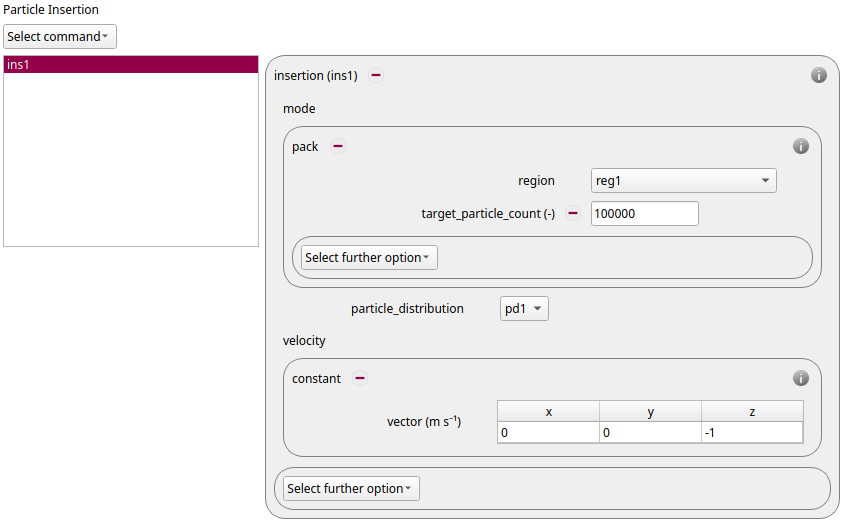
id |
|
mode |
|
region |
|
particle_distriubtion |
|
target_particle_count |
100000 |
velocity vector |
( 0, 0, -1) |
Simulation Control
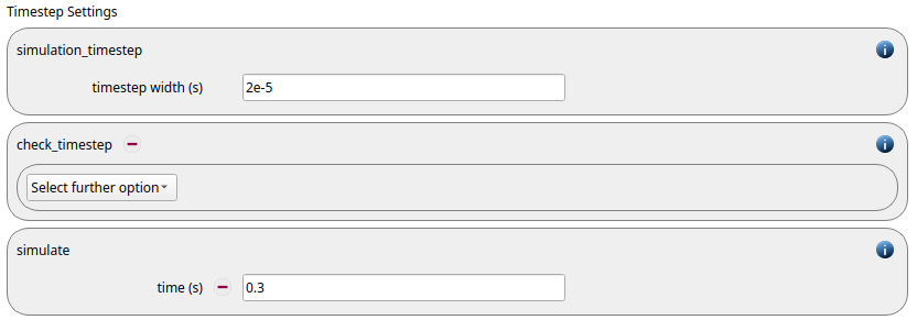
In this tab one first chooses the time step settings such as the desired simulation timestep of 2e-5 seconds and the total simulation time of 0.3 seconds. The check_timestep command is enabled by default. It throws a warning when the time step exceeds 10 % of the Rayleigh or the Hertz time step. These thresholds can be changed by setting an alternative value for hertz_fraction or rayleigh_fraction.
Output Settings
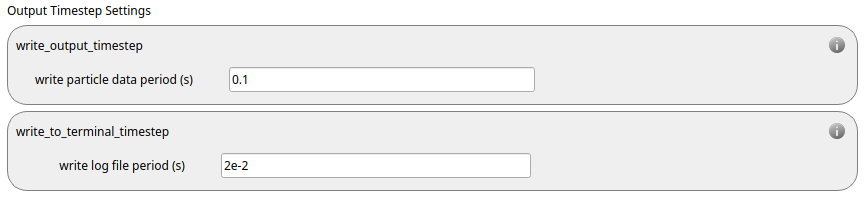
In this tab we first define the timestep width for the output to be 0.1 seconds and the terminal output to be 0.02 second:
The output_settings command takes care that all particle information and the meshes are written to files accordingly. Furthermore, it triggers the output of global quantities such as the kinetic energy of the particles or total normal and shear stresses onto meshes in the terminal. Please note that if the output of per-cell information on meshes such as velocity or stress are desired, the keyword mesh_properties has to be added and the required output has to be selected.
Preview
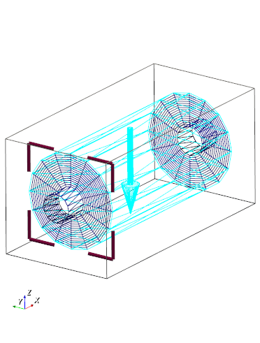
A preview of the full setup showing the domain, walls and meshes, along with the insertion region (and insertion direction) is visible in the preview window:
Running the Simulation
After saving the case we can change to the Simulation section. By hitting the Start button we can start running the GPU simulation.
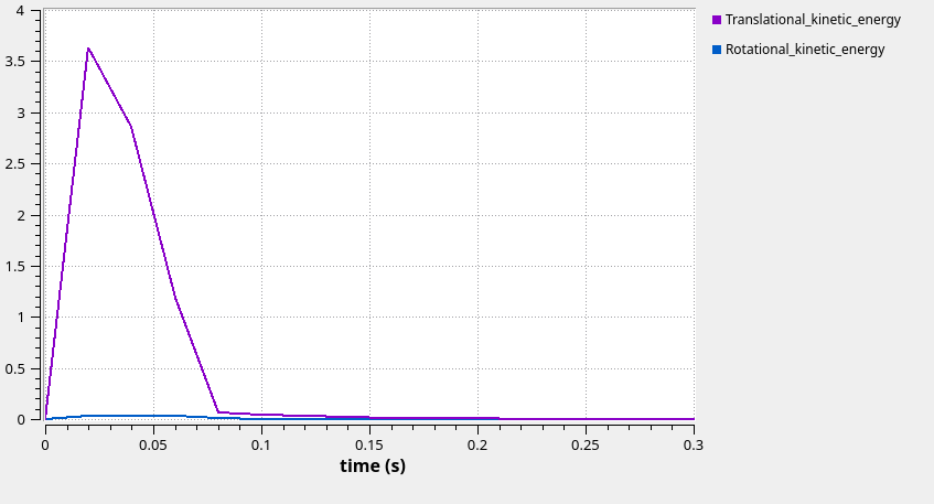
During the simulation, various quantities are displayed, such as the translational and rotational kinetic energy:
Postprocessing the Results
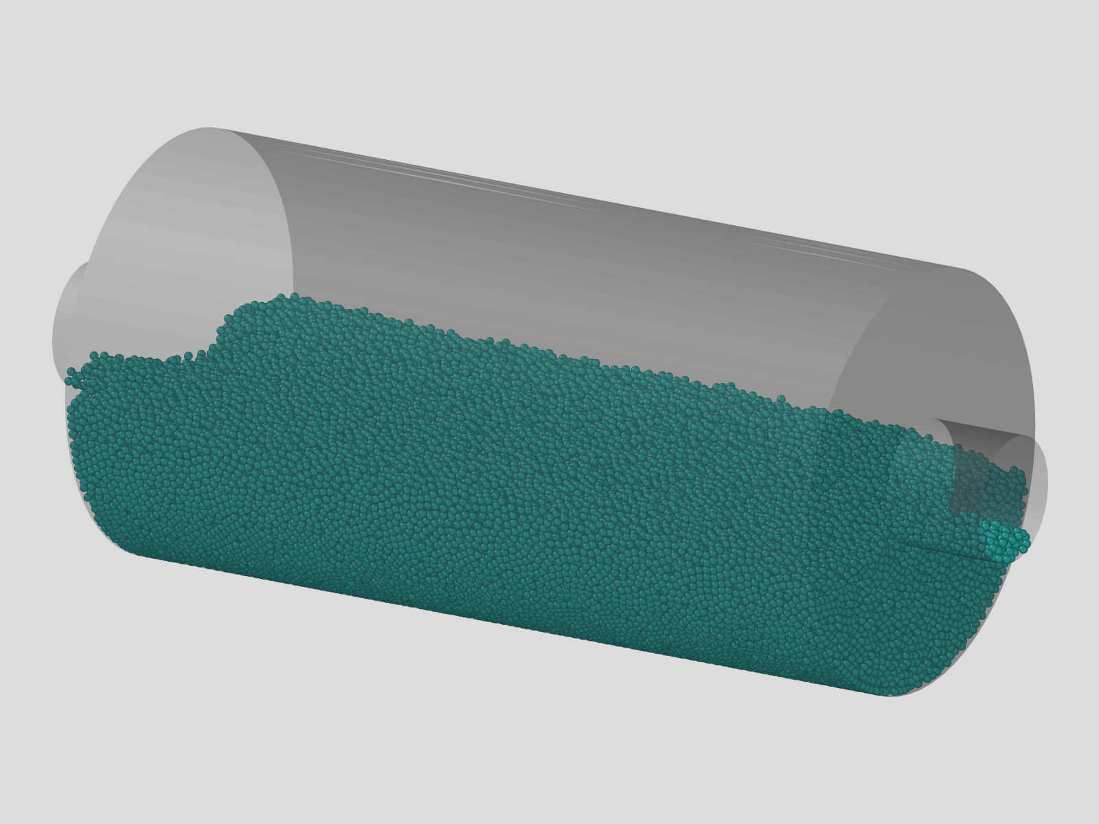
The results can be visualized in Ovito or Paraview. The image below shows the state of the simulation at the last time step:
Restarting & Continuing a GPU Simulation
Next, we create a derived simulation, in which we apply a shear force to the drum walls to mimic the rotational velocity.
Meshes & Regions
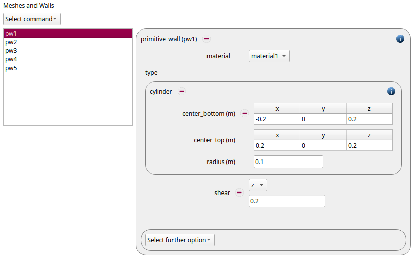
The property shear with a value of 0.2 is added to the main drum and the two disks (pw1, pw2, pw3):
Particles
In the Particles section, the insertion command is removed:

Simulation Control
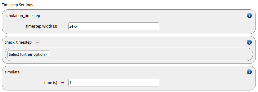
The total runtime is now extended to 1 second:
Running the Simulation
After saving the case we can change to the Simulation section. By hitting the Start button we can start running the GPU simulation.
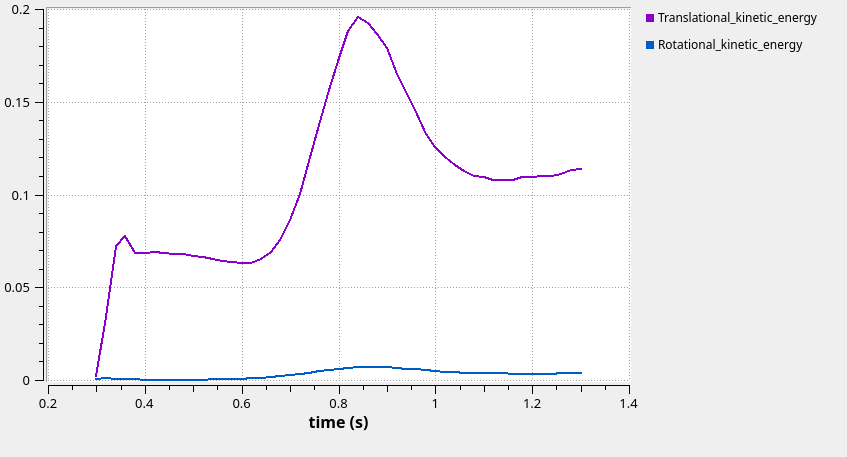
During the simulation, various quantities are displayed, such as the translational and rotational kinetic energy:
Postprocessing the Results
The results can be visualized in Ovito or Paraview. The image below shows the state of the simulation at the last time step: