Glowinski case with adaptive mesh refinement based on particle size

This setup uses the cell refinement indicator field obtained from IB voidfraction model to ensure that particles of different diameter are discretized with the same number of cells per diameter to fulfill the resolution requirements for resolved CFD-DEM simulations.

The setup is similar to the Glowinski setup and simulates two spheres falling in liquid, where the leading sphere is half the diameter of the trailing sphere.

Models used

This is a resolved CFD-DEM case using the immersed boundary method (IBM). Consequently models are used that take advantage of the resolved velocity and pressure field around the particle.

• Particle forces:

  • The drag force is computed by the Shirgaonkar model.

  • Alteration of effective gravity forces due the difference of fluid and particle densities is modelled by the IB variant of the Archimedes force model.

• Particles are mapped to CFD cells by a variant of the engine locateModel specifically tailored towards resolved CFD-DEM simulations.

• The voidfraction is computed by the IB voidfraction model accounting for large particles and using the writeRefinementIndicator setting.

• Mesh refinement is configured in dynamicMeshDict using the refIndicator field written by the IB voidfraction model:

  topoChanger
  {
      type            refinerCFDEM;
      libs            ( "libfvMeshTopoChangersCFDEM.so" );
      mover           none;
  
      refineInterval  1;
      field           "refIndicator";
      lowerRefineLevel 10;  // refine if refIndicator > 10
      upperRefineLevel 1e3; // refine if refIndicator < 1000
      unrefineLevel   0.9;  // unrefine only if refIndicator < 0.9
  
      nBufferLayers   2;
      maxRefinement   4;    // smaller particle needs refLevel 4, avoid excessive over-refinement
      maxCells        1000000;
  
      correctFluxes
      (
          ( phi U )
          ( phi_0 U )
      );
      dumpLevel       false;
  }
  

  In this application, a mesh refiner is used that preserves the refinement level until unrefinement is requested via the refinement indicator field.

• The case is run with cfdemSolverIB.

Superquadric variant

Note

This tutorial is included in and relies on functionality that is available in the CFDEMcoupling-Premium package.

A variant of the above case using cfdemSolverPimple with superquadric particles is also available. Very similar modeling approaches as for the case with spheres are used:

• Particle forces:

  • The drag force is computed by the Shirgaonkar model.

  • Alteration of effective gravity forces due the difference of fluid and particle densities is modelled by the IB variant of the Archimedes force model.

• Particles are mapped to CFD cells by a variant of the engine locateModel specifically tailored for superquadric particles.

• The voidfraction is computed by the IB voidfraction model accounting for large particles and using the writeRefinementIndicator setting.

  Note

  For the current setup, the definition of the minCellsPerParticle setting is crucial to get the desired behavior of adaptive refinement. In this case, particles are refined with at least 1000 cells and at max with 4000 cells.

• Resolved particles in the unresolved solver are modeled using a particular mesh motion model: IBParticle.

• Mesh refinement is configured in dynamicMeshDict using the refIndicator field written by the IB voidfraction model. The settings are identical to the settings for the spehrical case discussed above.

• The case is run with cfdemSolverPimple.

Results

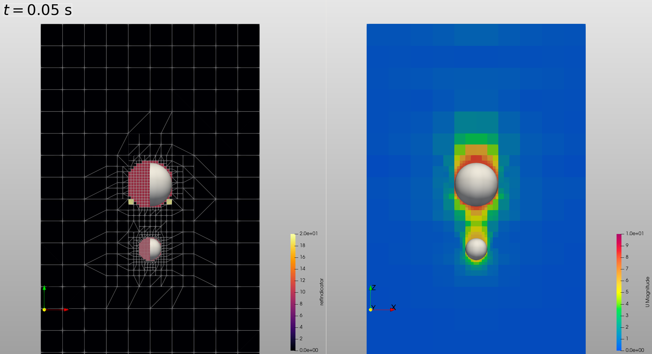
Figure 1: Left: Refinement indicator field and current mesh. The mesh shows that the leading smaller particle is discretized with smaller cells. Cells for the upper particle are marked for refinement. The particles are cut in half to show the refined mesh within the particles. Right: Fluid velocity.

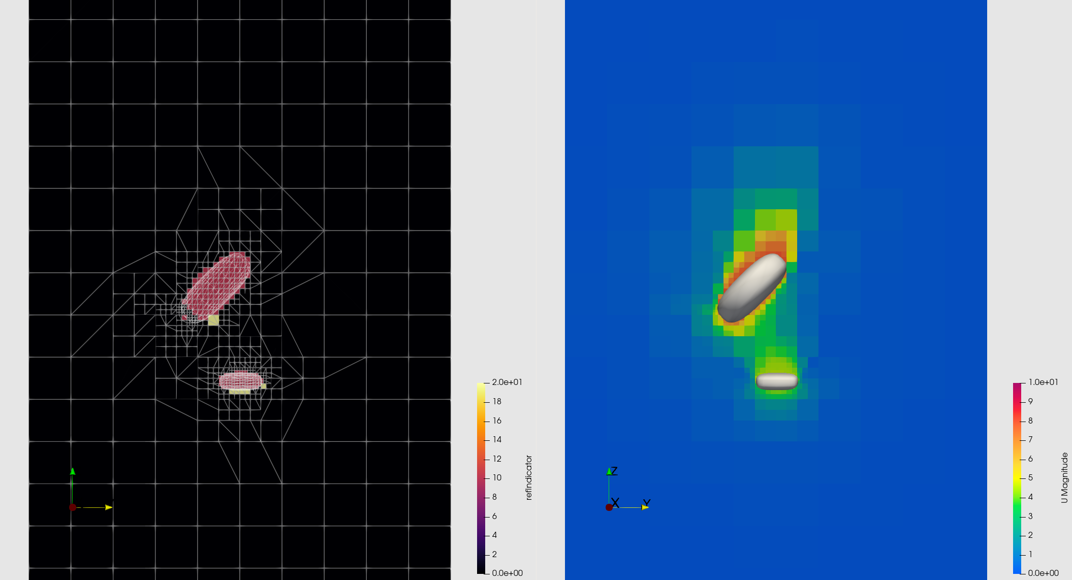
Figure 2: Same as above but for superquadric particles. The particles are displayed in a slightly different manner.