Setting up fastDEM simulations
Description:
This text describes how to perform “fast DEM” simulations in Aspherix®.
Introduction:
“Fast DEM” simulations are simulations of processes over longer time-scales compared to a typical DEM simulation. They can be applied to both steady-state processes or slightly instationary processes where the steady state experiences a time drift, e.g. when emptying a silo or due to chemical reactions.
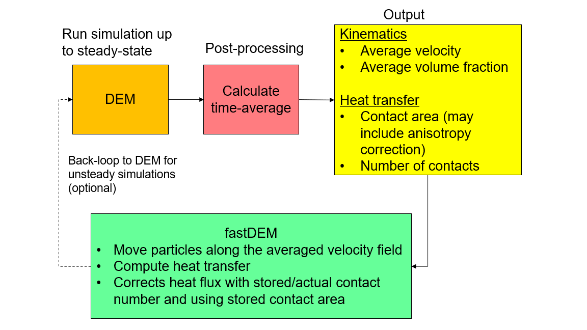
The concept of fast DEM involves several stages, as shown in the scheme below. First the simulation progresses towards a (pseudo) steady state, then averaging is performed, and then particle motion is projected forward, based on the average obtained. Optionally, in the case of time-drift of the steady state, the projection and DEM can be coupled together sequentially. In the projection phase, the particles experience a force that “drives” them towards the average obtained before. This relaxation of particle motion towards the average results has a stabilization effect, which allows much higher time-steps.
Detailed description:
The stages of a fast DEM simulation are shown in the table below. Every stage typically consists of a number of time-steps:
fast DEM stage |
description |
related commands |
1: Run simulation towards steady state |
Detect (pseudo) steady state using averaging method |
|
2: Obtain statistical averages of (pseudo) steady state |
Calculate averages, at least velocity and volume fraction |
|
3: Projection of particle motion |
Forward project particle motion, based on steady-state data |
|
optional 4: back-coupling to DEM |
run DEM time-steps to relax towards a new (pseudo) steady state, update statistics, then continue with stage 3 |
none |
In general, stages 1 and 2 can be combined into one. However, for a faster convergence detection it is advisable to reset the averaging after the initialization phase. This can be achieved using fix_modify average reset as described in fix ave/euler/custom/temporal/steadystate.
The optional stage 4 consists of several sub-stages:
DEM back-coupling sub-stages |
description |
4a: Relaxation towards valid packing |
After the projection stage, the packing configuration is not valid. Thus, first a valid packing / overlap structure has to be established |
4b: Relaxation towards new (pseudo) steady state |
Back-coupling to DEM is only necessary in cases where there is a time-drift for the steady state. Thus, the “physical” relaxation towards this new (pseudo) steady state is necessary |
4c: Update statistics |
Similar to stage 2, new or updated statistical data for the updated (pseudo) steady state is generated |
For step 4a, a blending of gravity forces and contact force (via fix relax/contacts) is recommended.
Practical tips
A number of practical tips can help you with setting up a fast DEM simulation:
Averaging of fix ave/euler/custom/temporal/steadystate can be turned on and off and reset using fix_modify average start/stop/reset
A fix relax/contacts is available to ease convergence behavior in step 4a
Typical/recommended differences between a “DEM stage” and “projection stage” are outlined below. For CFD-DEM and heat transfer, please see separate sections below.
Property or setting |
DEM stage |
projected DEM stage |
Young’s Modulus |
>= 5e7 Pa |
2e2 Pa |
neighbor list |
re-build using ‘skin’ setting when particle move too far |
fixed re-build every couple time-steps (e.g. 5) |
time-step size |
between 5%-20% of Rayleigh/Hertz times, see fix check/timestep/gran |
up to 50 % of these criteria (stabilization by relaxation towards equilibrium) |
number of time-steps per stage |
5000 to 50000 |
50-5000 |
forces from time-averaged fields |
no / not applicable |
yes, via fix addforce/steadystate |
body forces |
body forces (e.g. gravity) applied to the simulation |
no body forces applied to the simulation since effect contained in averaged velocity fields |
particle-particle forces |
yes |
yes, to prevent overpacking, but drastically reduced (lower Young’s Modulus) |
particle-wall forces |
yes |
yes, to prevent particles leaving domain due to round-off errors, but drastically reduced (lower Young’s Modulus) |
Heat transfer and fastDEM
In a CFD-DEM coupled simulation, the gas-particle convective heat transfer is not influenced by the packing mechanics and particle overlaps; hence, it can be safely applied directly.
The granular convective heat transport (i.e., the heat transported by moving particles) is also automatically resolved, provided that the fastDEM accurately resolves the velocity field and the density field in the simulation.
However, particle-particle and particle-wall heat conduction depend on the coordination number and the contact area, both of which are not valid in the projection phase of fastDEM. For this reason, it is suggested to calculate the conductive heat transfer as follows. As the DEM steady state is reached, it is necessary to generate the following statistics: average contact area (‘contact_area_conduction’), the average number of contacts (‘n_contacts_conduction’) and average particle-wall heat transfer coefficient (‘wall_heattransfer_coeff’). These are used to:
scale up/down the particle-particle heat transfer based on ratios of contact area and number of contacts in steady state stage vs. projection stage
calculate particle-wall heat transfer based on (T_wall - T_particle) * wall_heattransfer_coeff, assuming constant T_wall
Note that for particle-particle, the heat transfer is still computed based on particle-particle contacts. For the particle-wall heat transfer, the calculation is based on the cell-stored values for wall_heattransfer_coeff, i.e. particles will experience wall heat transfer in a cell close to the wall
The above-mentioned procedure can be implement using the following commands:
fast DEM stage |
description |
related commands |
1: Run simulation towards steady state |
not involved |
|
2: Obtain statistical averages of (pseudo) steady state |
calc statistics for ‘contact_area_conduction’ ‘n_contacts_conduction’ and ‘wall_heattransfer_coeff’ |
|
3: Projection of particle motion |
Use special fix to apply p-p and p-w heat conduction |
fix heat/gran/conduction/fast |
Note
The usage of different heat conduction model (namely, without area correction, with area correction and with modified area correction) does not affect the implementation in fastDEM, as the contact area is calculated once for all during the DEM phase and only the stored average value is used by fastDEM.
CFD-DEM and fastDEM (a.k.a. fastCFD-DEM)
The systematics of fastCFD-DEM is identical to fastDEM, with adding CFD coupling. The table below gives you an indication when CFD forces (i.e. any drag force, pressure gradient force, buoyancy force, lift force, etc.) should be used.
fast DEM stage |
CFD-DEM comments |
1: Run simulation towards steady state |
do include CFD forces |
2: Obtain statistical averages of (pseudo) steady state |
do include CFD forces |
3: Projection of particle motion |
do NOT include CFD forces, they are included in the steady state field already |
optional 4: back-coupling to DEM |
use full CFD forces for 4b and 4c, blending for 4a is recommended (similar to gravity and contact forces) |
Questions?
If any questions remain, contact us.