enable_one_way_coupling command
Purpose
Command for adding a drag force to particles. The command requires three types of user input:
the selection of a drag correlation,
the definition of the fluid and
other numerical settings.
A related command is enable_dem_drag, which is designed to
calculate drag force of particles in a coupled CFD-DEM simulation.
enable_dem_drag equals this command, except the fact, that
the fluid is defined by the coupled CFD simulation.
The drag force and torque acting on each particle can be visualized via the
properties id_dragforce_stored and id_dragtorque_stored.
For multisphere particles these properties are replicated onto every particle of a clump.
Syntax
enable_one_way_coupling keyword value
With the following keyword argument pairs:
Keywords related to fields settings
Keywords |
Description |
|---|---|
transient_fields |
bool (
yes or no) determining if fields change in timedefault:
no |
is_periodic_in_time |
bool (
yes or no) determining if transient fields are periodic in timedefault:
no, only read if transient_fields yes |
update_fields_every_time |
scalar value determining how often the field is interpolated in time
default: same as
update_every_time. only read if transient_fields yes |
binsize |
scalar or vector size of bins for structured grid used
mandatory
|
max_bins |
number of maximum bins in the grid that is used to interpolate the field values onto
default: 8,000,000
|
field_optimize_memory |
switch to deactivate partitioning of the field data to processes,
field_optimize_memory no may consume significantly more memorydefault:
yes |
check_mesh |
bool (
yes or no) determining if mesh size of specified field should be
checked against particle diameterdefault:
no |
interpolate_field_to_grid |
bool (
yes or no) determining if file is treated as exact representation
of the internal mesh or values are interpolateddefault:
yes |
interpolate_grid_to_particles |
bool (
yes or no) determining if field values are interpolated linearly
to the particle position or if the bin values are useddefault:
no |
U_fluid_file |
the file containing the data for the fluid velocity field
|
velocity_field_id |
the id of a eulerian_vector_field command
to use as velocity field
mutually exclusive with
U_fluid_file |
rho_fluid_file |
the file containing the data for the fluid density field
|
density_field_id |
the id of a eulerian_scalar_field command
to use as density field
mutually exclusive with
rho_fluid_file |
bool (
yes or no) determining if the elevation field must be used to set the densitydefault:
nooptional if
rho_fluid_file is set |
|
fluid_density_below_elevation |
scalar setting the fluid density below the elevation
mandatory, if
use_elevation is used; units: [mass/volume] |
fluid_density_above_elevation |
scalar setting the fluid density above the elevation
optional, if elevation is used; units: [mass/volume]
default:
0 |
use_relative_density |
bool (
yes or no) determining if the relative density must be added to the elevation valuesdefault:
nooptional if
use_elevation is used |
relative_density_field_name |
name defining the field that stores the relative density data
default:
RELATIVE DENSIT |
temperature_fluid_file |
the file containing the data for the fluid temperature field
|
temperature_field_id |
the id of a eulerian_scalar_field command
to use as temperature field
mutually exclusive with
temperature_fluid_file |
region |
the region’s id in which to apply the drag
default: entire simulation domain
|
U_fluid |
fluid velocity vector (ux, uy, uz)
; units: [length/time]
|
name defining the region’s id in which to apply the MRF mapping
|
|
scalar angular velocity of the rotating MRF region
mandatory, if
MRF_region set; units: [radians/time] |
Keywords related to physical properties and physics models
Keywords |
Description |
|---|---|
buoyancy |
bool (
yes or no) that switches on/off the buoyancy force for particles.
For coupled simulations (see enable_dem_drag command), fluid density field from
CFD is considered, otherwise the fluid density defined in this command is used.default:
no |
bool (
yes or no) activating correlations for compressible flowdefault:
no |
|
bool (
yes or no) activating calculation of rotational drag in compressible flowdefault:
no |
|
bool (
yes or no) activating the calculation of fluid particle heat transferdefault:
no |
|
fluid_viscosity |
scalar setting the kinematic fluid viscosity
mandatory; units: [area/time]
|
fluid_density |
scalar setting the fluid density
mandatory, if no density field is set; units: [mass/volume]
|
Drag related keywords
Keywords |
Description |
|---|---|
drag_model |
the drag model to use, see Drag model Specific Syntax
mandatory
|
implicit |
bool (
yes or no) to set if drag is handled implicitly,
i.e. as 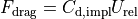 default:
no |
update_every_time |
scalar value or
auto defining the time interval to update the drag acting on particlesoptional
|
update_every_time_max |
scalar limiting the automatically calculated update interval
optional, available if
update_every_time auto. Must be > 0. |
nevery |
scalar defining the number of timesteps between drag updates. Alternative to
update_every_time.default:
1 |
max_acceleration_number |
scalar used to calculate the update interval
default:
0.05 , available if update_every_time auto. Must be in the range of [0.001, 1]. |
particle_templates |
list of particle_template command ids for which to apply the drag
default: all templates
|
bool (
yes or no) activating the use of an average voidfraction field,
which is computed internally based on the particle positionsdefault:
no |
|
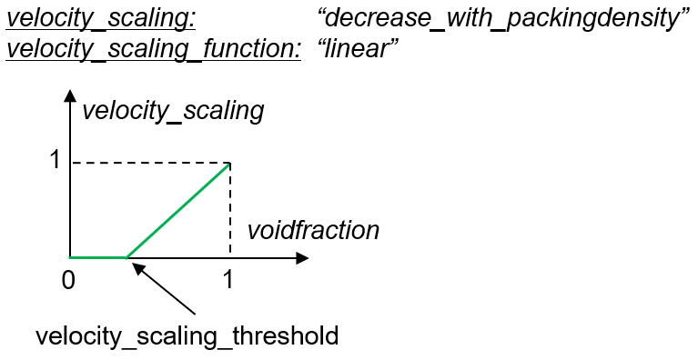
bool (
increase_with_packingdensity or decrease_with_packingdensity) activating the calculation of a local scaled velocity
from a superficial velocitydefault:
none , requires use_average_voidfraction |
|
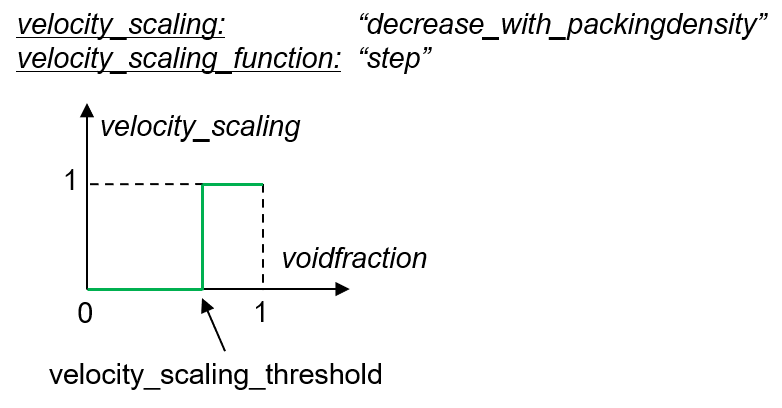
bool (
linear or step) selecting the function for calculation of a local scaled velocity
from a superficial velocitydefault:
none , requires velocity_scaling decrease_with_packingdensity |
|
scalar defining the threshold value of the
velocity_scaling_functiondefault:
0.82 , requires velocity_scaling decrease_with_packingdensity |
|
bool (
yes or no) the voidage correction based on DiFelice,
applicable only if a local voidfraction is available, either by using
enable_dem_drag command or by using use_average_voidfractiondefault:
yes |
|
attenuation_value |
scalar coefficient defining how drag is scaled
|
bool (
yes or no) activating the use of rotational torquedefault:
no |
Examples
enable_one_way_coupling drag_model Schiller_Naumann fluid_viscosity 0.0002 fluid_density 1000 region water
enable_one_way_coupling drag_model const_Cd Cd 1.5 fluid_viscosity 0.0002 fluid_density 1000 U_fluid (1, 0, 0)
enable_one_way_coupling drag_model Schiller_Naumann fluid_viscosity 0.002 fluid_density 10 region r2 &
    binsize 0.1 U_fluid_file data/cfd_field
enable_one_way_coupling drag_model Schiller_Naumann &
   fluid_viscosity 0.002 fluid_density 10 region r2 binsize 0.1 U_fluid_file data/cfd_field &
   MRF_region MRFregion MRF_angular_velocity 1
enable_one_way_coupling drag_model DiFelice implicit no &
   interpolate_field_to_grid no interpolate_grid_to_particles yes &
   region region_part1 binsize (200,200,15) &
   update_every_time auto update_every_time_max 1e-3 &
   attenuation_value 0.1 transient_fields yes fluid_viscosity 1e-6 &
   U_fluid_file data/ocean/sequence.file &
   rho_fluid_file data/ocean/sequence.file use_elevation yes &
   fluid_density_below_elevation 1000 buoyancy yes
Field specification
This command reads field data from csv, vtk, and vtu files. For more detailed
information on how to format files and similar, see eulerian_scalar_field and eulerian_vector_field commands.
This command will internally create the eulerian_scalar_field and eulerian_vector_field commands as needed. Hence, there is no need to manually create these commands, unless these fields are to be defined with different settings, e.g. with different binsize or mixing steady and transient fields.
Drag model Specific Syntax
drag_model drag_correlation
This command adds the following drag force to particles:
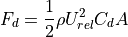
where  is the particle’s cross-sectional area,
  is the relative
velocity of particle and fluid,
is the relative
velocity of particle and fluid,  is the fluid density.
Depending on the
is the fluid density.
Depending on the drag_correlation  is calculated differently, see the definitions below.
Optionally, when setting rotational_torque, a rotational torque can be calculated:
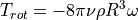
where  is the particle rotation (neglecting fluid rotation),
  is the
kinematic fluid_viscosity of the fluid, is the fluid density and
is the
kinematic fluid_viscosity of the fluid, is the fluid density and  the
radius of the volume equivalent sphere. By default the rotational torque is neglected, unless
the user specifies differently).
the
radius of the volume equivalent sphere. By default the rotational torque is neglected, unless
the user specifies differently).
Voidfraction corrections
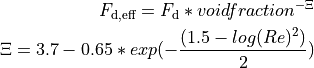
Depending on use_voidage_correction, and if a local voidfraction is available
(either by using enable_dem_drag command, or by using use_average_voidfraction),
the dragforce acting on each particle  is scaled to account for the presence
of other particles. This is known as voidage correction or swarm effect.
is scaled to account for the presence
of other particles. This is known as voidage correction or swarm effect.
All components of the force: drag, lift and pitch torque (if the drag model provides that) are scaled equally.
The keyword use_average_voidfraction, is used to calculate a local average voidfraction field,
which is computed internally based on the particle positions. This voidfraction field is automatically written
via output_settings command as Eulerian Field. Through the use_voidage_correction, the local voidfraction is
is used to account for swarm effect. This approach could be called a 1.5 way coupling.
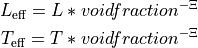
Velocity scaling
The keyword velocity_scaling (to be used in combination with use_average_voidfraction),
is used to scale the provided velocity field (or single vector U_fluid)
 , where the scaling is based on a local
average voidfraction.
There are models for two different applications: “confined flow” and “unconfined flow”:
, where the scaling is based on a local
average voidfraction.
There are models for two different applications: “confined flow” and “unconfined flow”:
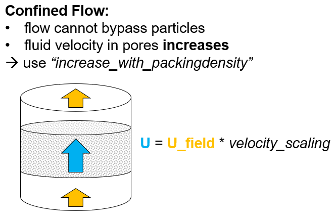
For “confined flow” you should use the option: increase_with_packingdensity.
The velocity seen by the particles is then increased from a “superficial velocity”
to an “interstitial velocity”.
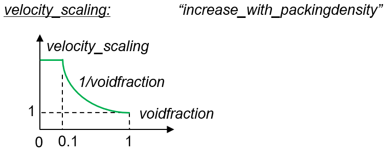
Velocity scaling function
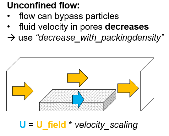
For “unconfined flow” you should use the option: increase_with_packingdensity.
The velocity seen by the particles is then decreased from a superficial velocity
to an velocity inside the particle packing. Here it is assumed that the flow can
easily bypass the particles and therefore hardly any velocity is present inside a
particle packing. For this option, two scaling functions velocity_scaling_function are available:
linear and step. Additionally the user can specify the “velocity_scaling_threshold” value.
Avilable drag correlations for spheres
The following drag models are designed for spheres but an application to nonspherical particles is possible (see next section). Note that the coarsegraining command can be used in combination with these drag models.
Drag correlation: const_Cd
const_Cd      (mandatory) keyword to select the drag correlation
Cd            (mandatory) scalar value of drag coefficient (dimensionless)

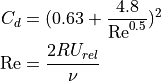
Drag correlation: Schiller_Naumann
Schiller_Naumann (mandatory) keyword to select the drag correlation
where  is the Reynolds Number, is the
kinematic fluid_viscosity of the fluid and R is the particle
radius.
is the Reynolds Number, is the
kinematic fluid_viscosity of the fluid and R is the particle
radius.
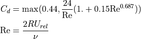
Drag correlation: DiFelice
DiFelice (mandatory) keyword to select the drag correlation
where is the Reynolds Number, is the
kinematic fluid_viscosity of the fluid and R is the particle
radius.
Available drag correlations for non-spherical particles
All drag correlations described in the previous section are designed for the application to spheres and might, depending on the actual shape of the non-spherical particles, lead to inaccurate results when used with multispheres, superquadrics or arbitrary particles. However, also these sphere drag models can be applied to non-spherical particles. A drag model that has been concipated specifically for non-spherical particles is the Zastawny drag correlation (see below).
General parameters for nonspherical drag models
hydraulic_diameter        (mandatory if use_point_cloud is yes) list of scalars defining
                            the hydraulic diameter of each particle_template ( units)
use_point_cloud yes       keyword/style pair
use_point_velocity        (optional if use_point_cloud is yes, default false) bool defining wether each point should use the centre of mass velocity of the clump, or its point velocity.
                Using the point velocity will lead to an additional rotational torque.
point_cloud_file          (mandatory if use_point_cloud is yes) list of files defining the point cloud
                            of each particle_template (x y z weight)
point_cloud_scaling       list of scalars defining the geometric scaling of each of each point_cloud_file data
units)
use_point_cloud yes keyword/style pair
use_point_velocity (optional if use_point_cloud is yes, default false) bool defining wether each point should use the centre of mass velocity of the clump, or its point velocity.
Using the point velocity will lead to an additional rotational torque.
point_cloud_file (mandatory if use_point_cloud is yes) list of files defining the point cloud
of each particle_template (x y z weight)
point_cloud_scaling list of scalars defining the geometric scaling of each of each point_cloud_file data
Example for a multisphere particle and a possible point cloud file:
Multisphere defintion file:
0 -0.01 -0.01  0.01
0  0     0     0.01
0  0     0.01  0.01
0  0     0.02  0.01
0  0.01  0.03  0.01
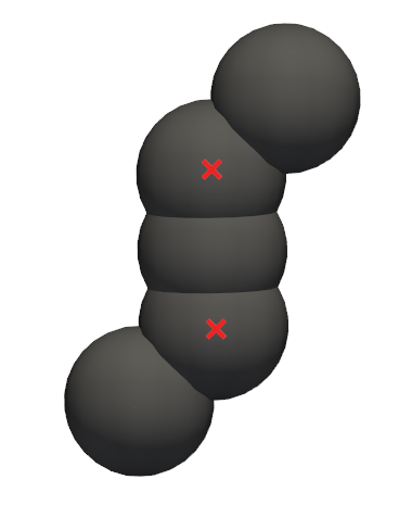
Pointcloud definition of non-spherical particles
For non-spherical particles it is possible to provide a list of points for every particle template
that will be used as base for the drag calculation instead of using the center of mass only
(use_point_cloud yes, point_cloud_files). The point cloud for each particle template uses the
same coordinate system as the particle template.
Note that the coarsegraining command can be used in combination with these drag correlations for non-spherical particles. But beware that while translatory motion will be well captured, the rotational motion of a non-spherical coarsegrained particle will be different to an original sized non-spherical particle!
Example for a pointcloud file, where the first three entries are the x, y and z coordinates of a point in the point cloud and the last entry is the respective weight for this point:
0  0  0     0.5
0  0  0.02  0.5
The weight is typically unity and is a relative measure (normalized by the sum of all point weights in that clump) increasing the impact of one point over others, meaning that the exact value is of lesser importance but the ratio of values among different points matters. If the weight for all points is identical, then all these points will contribute equally to the clump’s drag force.
If rotational_torque yes, then the drag / lift / torque are not only calculated for the
centre of mass of a particle, but for the entire point cloud.
Therefore a point_cloud_file is defined in the particle’s frame of reference. The points must
be defined relative to the centre of mass of the clump, and that the clump must be defined so
that the x,y,z are aligned with its eigenvectors. For each of the N points the drag F / lift
L / torque T of point i is calculated separately using the local fluid velocity and then
summed to the total particle force.
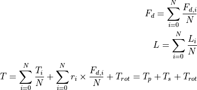
The torque therefore has three components: the pitch torque, the torque due to velocity gradients seen by a non-spherical particle and the rotational torque.
Drag correlation: Zastawny
Drag model for non-spherical particles, according to Zastawny, M., Mallouppas, G., Zhao, F., & Van Wachem, B. (2012). Derivation of drag and lift force and torque coefficients for non-spherical particles in flows. International Journal of Multiphase Flow, 39, 227-239.
Depending on the model parameters, the drag of various shapes such as ellipsoids, discs or fibers can be modelled. The model requires using multisphere particles.
Note
The implementation assumes that the x-direction (ex_space) of the particle_template command is the major axis of the body. For a disc like shape this means x-direction is in the disc plane, choose z-direction as disc normal.
Additional keayword argument pairs (all mandatory):
Zastawny keyword to select the drag correlation a0 - a8 lists of scalars, each defining the model parametersaiof eachparticle_templateb1 - b10 lists of scalars, each defining the model parametersbiof eachparticle_templatec1 - c10 lists of scalars, each defining the model parametersciof eachparticle_template
When using the Zastawny drag correlation, the usage of the keywords hydraulic_diameter,
use_point_cloud yes and point_cloud_file is mandatory.
Example:
enable_one_way_coupling drag_model Zastawny &
    fluid_viscosity 0.002 fluid_density 10 &
    update_every_time auto &
    U_fluid_file data/cfd_field binsize 0.1 &
    region r2 &
    use_point_cloud yes &
    hydraulic_diameter {7.213282e-03,7.213282e-03} &
    point_cloud_file {data/pointCloud.txt,data/pointCloud.txt} &
    a0 {2.0, 2.0}       a1 {5.1, 5.1}        a2 {0.48, 0.48}    a3 {15.52, 15.52}   &
    a4 {1.05, 1.05}     a5 {24.68, 24.68}    a6 {0.98, 0.98}    a7 {3.19, 3.19}     &
    a8 {0.21, 0.21}
    b1 {6.079, 6.079}   b2 {0.898, 0.898}    b3 {0.704, 0.704}  b4 {-0.028, -0.028} &
    b5 {1.067, 1.067}   b6 {0.0025, 0.0025}  b7 {0.818, 0.818}  b8 {1.049, 1.049}   &
    b9 {0, 0}           b10 {0, 0} &
    c1 {2.078, 2.078}   c2 {0.279, 0.279}    c3 {0.372, 0.372}  c4 {0.018, 0.018}   &
    c5 {0.98, 0.98}     c6 {0, 0}            c7 {0, 0}          c8 {1, 1}           &
    c9 {0, 0}           c10 {0, 0}
Drag correlation: other_proprietary_models
drag_correlation   ...
...   ...
Rotating stationary field
In case both a MRF_regio and MRF_angular_velocity are specified on top of a static field,
the Multiple Reference Frame (MRF) feature is enabled. This feature
allows you to specify a rotating reference frame inside your otherwise
static fluid field. The particles in a MRF region are mapped to a
rotating coordinate system and the particle drag is computed correctly
for the rotating fluid velocity field in this region. An example for
such a region would be a spinning fan.
MRF_region (mandatory) name defining the region's id in which to apply the MRF mapping MRF_angular_velocity (mandatory) scalar angular velocity of the rotating MRF region (units)
The MRF_region keyword is used to specify the name of a region that
must be of either style cone or cylinder. The rotation
axis and center of rotation is derived from this region. Note, it is
not allowed that this region varies in size and that ‘side out’ is
used. The MRF_angular_velocity keyword specifies the angular
velocity of the rotating region and is taken with respect to the axis
of the region and the right-hand-rule.
Warning
MRF is not available for transient fields, i.e. when U_fluid_file or
transient_fields yes are set.
Drag calculation for compressible flow
If setting, compressible_flow yes, drag is calculated for compressible flow and
a temperature field must be provided by either setting the temperature_fluid_file
or the temperature_field_id keywords.
The temperature field is used to calculate the local viscosity using the
Sutherland law:
visc = visc_ref * (tf / Tref)^1.5 * (Tref + S) / (tf + S)
with tf being the local fluid temperature, visc_ref the dynamic viscosity at reference temperature Tref, and S the Sutherland temperature.
These properties may be set by the following keywords:
Keywords |
Description |
|---|---|
sutherland_ref_visc |
scalar setting the (dynamic) reference viscosity
default:
18.27e-6; units: [Pa s] |
sutherland_ref_temp |
scalar setting the reference temperature
default:
291.15; units: [temperature] |
sutherland_S |
scalar setting the Sutherland constant
default:
120.0; units: [temperature] |
Drag and torque calculation for compressible flow
If setting, compute_dragtorque yes, in addition to the calculation of a drag force,
a drag torque is calculated which decreases the particles rotational velocity
relative to the local fluid vorticity and a Magnus force may be computed.
The following keywords may be set:
Keywords |
Description |
|---|---|
compute_rotational_drag |
bool (
yes or no) activating the calculation of rotational dragdefault:
no |
compute_magnus_lift |
bool (
yes or no) activating the calculion of a Magnus forcedefault:
no |
If compute_rotational_drag yes, the rotational drag is computed as:
8 * pi * nu * rhoF * radius^3 * omegaRel
If compute_magnus_lift yes, the Magnus lift force is computed as:
pi * rhoF * radius^3 * (uRel x omegaRel)
with the local fluid density rhoF, the fluid viscosity nu, the relative particle velocity uRel, the relative particle rotational velocity omegaRel, and the cross product operator x.
Particle-fluid heat transfer calculation
If enable_particle_fluid_heat_transfer yes, then also fluid-particle heat transfer
is considered. This setting requires an enable_heat_transfer command to be defined
before. Moreover, a temperature field must be defined by either setting the
temperature_fluid_file or the temperature_field_id keyword.
The following additional keywords may be set:
Keywords |
Description |
|---|---|
fluid_thermal_conductivity |
the fluid thermal conductivity
default:
1e-3; units: [energy / (time length temperature)] |
fluid_prandtl |
the fluid Prandtl number
default:
1 |
voidfraction_file |
file to read voidfraction from
|
voidfraction_value |
scalar value for voidfraction
default:
1, mutually exclusive with voidfraction_file |
heat_transfer_correlation |
the correlation to use, see below
mandatory, either
Whitaker, LiMason, or Deen |
attenuate_heat_transfer |
scalar coefficient defining how heat transfer is scaled
default:
1 |
conductivity_evaporation_correction |
correction function for heat transfer due to evaporation
default:
none, either simple or Bird |
conductivity_evaporation_correction_Tbase |
the model function base temperature
default:
1, only used if conductivity_evaporation_correction Bird |
conductivity_evaporation_correction_factor |
the factor of fluid thermal conductivity at evaporation temperature
default:
1, only used if conductivity_evaporation_correction Bird |
conductivity_evaporation_correction_exponent |
the model function exponent
default:
1, only used if conductivity_evaporation_correction Bird |
The resulting heat flux depends on fluid and particle temperature.
The heat flux is computed via a Nusselt number correlation selected by the heat_transfer_correlation
keyword with the following options:
Heat transfer correlations
Whitaker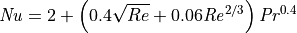
LiMasonCorrelation of Li and Mason (2000) A computational investigation of transient heat transfer in pneumatic transport of granular particles. Pow.Tech 112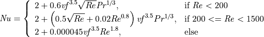
DeenCorrelation of N.G. Deen et al. (2014) Review of direct numerical simulation of fluid–particle mass, momentum and heat transfer in dense gas–solid flows. Chemical Engineering Science 116, 710–724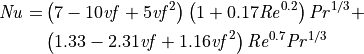
where vf is the void fraction, Pr is the fluid Prandtl number and Re is the particle Reynolds number:
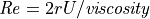
with viscosity defined by the fluid_viscosity keyword.
The voidfraction to use, may be defined by the corresponding keywords, either
voidfraction_file or voidfraction_value.
Evaporation correction
In case the particles contain evaporating liquid, the fluid thermal conductivity
can be corrected using conductivity_evaporation_correction simple by the model function
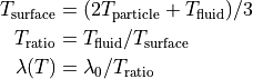
or by the approximated Bird correction using conductivity_evaporation_correction Bird:
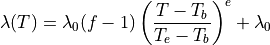
with
 : the liquid evaporation temperature as specified by the
 tempEvaporatematerial property : the fluid thermal conductivity set using the
 fluid_thermal_conductivitykeyword : the factor of fluid thermal conductivity at evaporation temperature, i.e.
  , specified by the
 conductivity_evaporation_correction_factorkeyword : the model function base temperature set using the
 conductivity_evaporation_correction_Tbasekeyword : the model function exponent set using the
 conductivity_evaporation_correction_exponentkeyword
The exponent must not be negative and the expression is limited to values in the interval
![[T_b, T_e]](_images/math/308604da9831f643e5f578f46ef5f160d4c5a31c.png)
Restrictions
A particle_template must be defined before this command.
The keyword use_superficial_velocity is legacy and has been replaced by velocity_scaling