enable_heat_transfer command
Purpose
Command for calculating particle-particle and particle-wall heat transfer and temperature update for the particle(s) and/or wall (via mesh_module_heattransfer).
Note
This command is supported by Aspherix GPU.Syntax
enable_heat_transfer keyword value
Keywords:
Keyword |
Description |
|---|---|
obligatory, initial temperature of the particles
units: [temperature]
|
|
id |
user-assigned name for the command call |
particle_group |
ID of the group of particles on which the command is applied
default: all
|
available options:
yes or nodefault:
no |
|
maximum_particle_temperature |
maximum temperature of the particles
units: [temperature]
|
number of shells used to discretize each particle
default: 1
|
|
available options:
yes or nodefault:
no |
|
available options:
yes or nodefault:
no |
|
available options:
yes or nodefault:
no |
|
available options:
yes or nodefault:
no |
Keywords for enable_radiation yes
Keyword |
Description |
|---|---|
filename of the view factors file |
|
emissivity of the particles
units [power/length^2]
|
|
relative cutoff radius for the radiation omdel
units [-]
|
|
number of interpolation points in the view factors data
default: 20
|
|
particle radius taken for area calculation
units [length]
|
Examples
enable_heat_transfer initial_particle_temperature 273.15
enable_heat_transfer particle_group my_particles id my_transfer initial_particle_temperature 273.15 &
  maximum_particle_temperature 373.15
enable_heat_transfer initial_particle_temperature 273.15 store_contact_data yes
enable_heat_transfer initial_particle_temperature 400 number_of_shells 20
enable_heat_transfer initial_particle_temperature 273.15 enable_radiation yes view_factors_file vf.csv emissivity 0.65 max_relative_radius 4 interpolation_resolution 15 add_external_heatflux yes
Associated material properties
Material properties
thermalConductivity( ): thermal conductivity of a material [power / length temperature]
thermalCapacity( ): thermal (specific) capacity of a material [energy / mass temperature]
youngsModulusOriginal( ): original Young’s modulus of each material [pressure] (required if
 area_correction yesis used in the particle_contact_model command)
Material interaction properties
ht_modification( ): modifier for contact area calculation [-] (required if
 modified_area_correction yesis used in the particle_contact_model command)
Description
This command computes the particle-particle and particle-wall heat transfer due to interaction and updates the particle temperature. To control the behaviour of this model several keywords can be used and their behaviour is detailed below.
The obligatory initial_particle_temperature defines the initial temperature
of the particles.
The temperature inside the particle can be updated using two different models.
The default uniform temperature model assumes a constant temperature throughout
the particle and can be chosen by using number_of_shells 1. The alternative
shell model discretizes the particle into a number of shells specified by
number_of_shells N (N > 1) and computes the corresponding heat transfer
inside the particle.
Uniform temperature model
This model chosen with number_of_shells 1 assumes a constant temperature
inside a particle and updates the temperature based on the following model
[1]
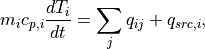
where  is the mass,
  is the heat capacity,
 is the temperature and
  is the heat source (or
sink) for the i-th particle. The heat flux
is the heat source (or
sink) for the i-th particle. The heat flux  stemming from
conduction via inter-particle contacts is summed over all contacts (index
j) of particle i.
stemming from
conduction via inter-particle contacts is summed over all contacts (index
j) of particle i.
Shell temperature model
This model discretizes the interior of each particle into N radial shells and computes the heat transfer between these shells inside each particle.
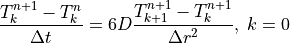
Heat conduction and temperature update are solved according to following 1D heat equation
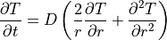
where the temperature inside a particle does depend only on the radial distance, but not on the azimuthal and polar angles. D is the thermal diffusivity:

Dividing the spherical particle of radius  into
into  spherical shells and discretizing the heat equation using the implicit
integration scheme gives us
spherical shells and discretizing the heat equation using the implicit
integration scheme gives us

where the temperature field is defined at the border points between shells
(grid points) and is the number of the grid point. Note that this
scheme is valid only for internal grid points ( ).
).
In order to avoid singularity problem for the particle center
( ) the L’Hopital’s rule is applied to the original heat
equation, leading to
) the L’Hopital’s rule is applied to the original heat
equation, leading to
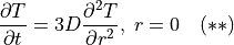
Applying the auxiliary point method:
the discretization of Equation (**) for  leads to
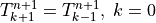
For the outer grid point ( ), Neumann boundary condition is
applied and discretized by introducing the auxiliary point
), Neumann boundary condition is
applied and discretized by introducing the auxiliary point  :
:
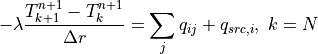
where is the heat source (or sink) for the i-th
particle. The heat flux stemming from conduction via
inter-particle contacts is summed over all contacts (index j) of particle
i. The value for the auxiliary point ( ) can be expressed and
substituted in Equation (*).
) can be expressed and
substituted in Equation (*).
As a result, the above mentioned equations provide a system of  linear equations with unknown values for temperature inside a
particles at the next time step:
linear equations with unknown values for temperature inside a
particles at the next time step:
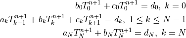
This system is then solved using the tridiagonal matrix algorithm.
To make particles adiabatic (so they do not change the temperature), do not include them in the fix group. However, heat transfer is calculated between particles in the group and particles not in the group (but temperature update is not performed for particles not in the group). Thermal conductivity and specific thermal capacity must be defined for each atom type used in the simulation by means of fix property/global commands:
fix id all property/global thermalConductivity peratomtype value_1 value_2 ...
(value_i=value for thermal conductivity of atom type i)
fix id all property/global thermalCapacity peratomtype value_1 value_2 ...
(value_i=value for thermal capacity of atom type i)
To set the temperature distribution for a group of particles, you can use
the set command with keyword property/atom and values temp_array T_0 T_1
.. T_N. T_0 T_1 .. T_N are the temperature values for grid
points respectively you want the particles to have. To set heat sources (or
sinks) for a group of particles, you can also use the set command with the
set keyword: property/atom and the set values: heatSource h where
 is the heat source value you want the particles to have (in
Energy/time units). A negative value means it is a heat sink. Examples
would be:
is the heat source value you want the particles to have (in
Energy/time units). A negative value means it is a heat sink. Examples
would be:
set region halfbed property/atom temp_array 800. 800. 800. 800. 800. 800. 800. 800. 800. 800. 800. 800. 800. 800. 800. 800. 800. 800. 800. 800. 800.
set region srcreg property/peratom heatSource 0.5
The heat flux between two particles or a particle and a wall in contact is defined as
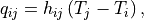
where the heat transfer coefficient  is calculated from the individual thermal conductivities
and a contact area
is calculated from the individual thermal conductivities
and a contact area  as
as
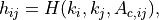
where  depends on whether a particle-particle or particle-wall contact is considered.
Details on heat transfer coefficient calculation
The heat transfer coefficient for particle-particle interactions
is calculated from the individual thermal conductivities
as follows
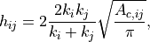
where is the contact area between the i-th and the
j-th particle. Note that for these relations to be valid, in general the
temperatures must be defined far away from the point of contact.
Similarly, the particle-wall heat flux can be written as
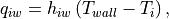
where the particle-wall heat transfer coefficient  for
particle i and a wall is calculated as follows:
for
particle i and a wall is calculated as follows:
where  is the particle thermal conductivity and
  is the contact area between the i-th and the wall. The difference between
these two equations for the heat transfer coefficient comes from the
definition of the (discrete) temperature locations. For particle-particle
interactions these are both far away for the point of contact. However, for
particle-wall interactions only one the particle temperature is defined far
away, while the wall temperature is defined at the point of contact.
Therefore, if the particle and wall would have identical thermal
conductivities, these two equations will lead to different heat transfer
coefficients (
is the contact area between the i-th and the wall. The difference between
these two equations for the heat transfer coefficient comes from the
definition of the (discrete) temperature locations. For particle-particle
interactions these are both far away for the point of contact. However, for
particle-wall interactions only one the particle temperature is defined far
away, while the wall temperature is defined at the point of contact.
Therefore, if the particle and wall would have identical thermal
conductivities, these two equations will lead to different heat transfer
coefficients ( ). The factor 2 compensates for the
distance change between the (discrete) temperature locations, which for
particle-particle interactions is 2 times the distance for particle-wall
interactions. Another way to look at it is to consider a pile of 2
particles squeezed between two flat horizontal walls with different
temperatures. To obtain (vertically) a linear temperature gradient (which
implies a constant heat flux value between the walls), the
particle-particle and particle-wall temperature differences should be equal
to
). The factor 2 compensates for the
distance change between the (discrete) temperature locations, which for
particle-particle interactions is 2 times the distance for particle-wall
interactions. Another way to look at it is to consider a pile of 2
particles squeezed between two flat horizontal walls with different
temperatures. To obtain (vertically) a linear temperature gradient (which
implies a constant heat flux value between the walls), the
particle-particle and particle-wall temperature differences should be equal
to 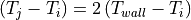 .
Therefore, the shown heat transfer coefficients and temperature differences
will lead to a constant heat flux value across the domain (it is not be
affected by the interaction type: particle-particle or particle-wall):
.
Therefore, the shown heat transfer coefficients and temperature differences
will lead to a constant heat flux value across the domain (it is not be
affected by the interaction type: particle-particle or particle-wall):
 .
.
To make particles adiabatic (so they do not change the temperature), do not include them into the group addressed by group-ID. Independently from that, heat transfer is calculated between particles in the group and particles not in the group (but temperature update is not performed for particles not in the group). Thermal conductivity and specific thermal capacity must be defined for each atom type used in the simulation by means of material_properties command:
material_properties glass thermalConductivity 100 thermalCapacity 1 ...
To set the temperature for a group of particles, you can use the set command
with keyword property/atom and values Temp T. T is the temperature value
you want the particles to have. To set heat sources (or sinks) for a group of
particles, you can also use the set command with the set keyword:
property/atom and the set values: heatSource  , where
is the heat source value you want the particles to have (in
Energy/time units). A negative value means it is a heat sink. Examples would
be:
, where
is the heat source value you want the particles to have (in
Energy/time units). A negative value means it is a heat sink. Examples would
be:
set region halfbed property/peratom Temp 800.
set region srcreg property/peratom heatSource 0.5
The calculation of the contact area can be influenced by
several keyword settings of the particle_contact_model command to adjust the particle shapes, surface
properties and other relevant effects.
Details on contact area calculation
Please see the documentation of the particle contact model and wall contact model
commands. They have several keywords to control the details of the contact area calculations. Additionally, the
area_shape keyword is described here below.
Area shape
If area_shape is set to circle [default] then the particle-particle
() and particle-wall () heat transfer
coefficients are calculated as indicated in the equations above. Note that
circle is in general appropriate, but for certain reasons (backward
compatibility) another setting might be chosen. If this keyword is set to
square, then  is replaced by 4 in the equation. If this
keyword is set to
is replaced by 4 in the equation. If this
keyword is set to legacy, then is omitted in the equation
(replaced by 1). As the thermal conductivity is a calibration parameter
this is not a big issue, as switching from the legacy representation
(default up to Aspherix 5.3.x) to the physically more correct circle
representation (default from Aspherix 5.4) can be achieved by dividing the
current thermal conductivities by  .
.
In case enable_radiation is set to yes a radiation model based on local void fractions and particle distance is employed using view factors read from a file.
Radiation model
The model that was implemented is based on the work of Johnson et al. [2].
It defines the heat transferred from a particle  to a particle
 as
as
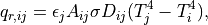
where  is the
 emissivity of the particles which can be
specified with the corresponding keyword.  is the average
surface area of the two particles and
is the average
surface area of the two particles and  the Stefan Boltzmann
constant. and
the Stefan Boltzmann
constant. and  are the absolute temperatures of the
two praticles and
are the absolute temperatures of the
two praticles and  the view factor which depends on the
average local volume fraction
the view factor which depends on the
average local volume fraction  and the
distance between the two particles centroids
and the
distance between the two particles centroids  .
.
The area can also be set as constant for all contacts using
the apparent_particle_radius keyword, which defines the area based on
this radius value.
The total heat transferred to a particle is calculated as the sum of all
particle-particle heat rates where the particle centroid distance is less
than a certain value  . This is either defined via the
max_relative_radius keyword or taken from the largest radius listed in
the view_factors_file. This file is a csv file with comma (or space)
separated values. The first line must be a header which must define the
first column as ‘r’ and all subsequent columns via their corresponding
volume fraction. The rows of the data that will follow below specify the
relative radius in the first row and then the view factor corresponding to
that radius and the volume fraction. As very basic file could look like:
r, 0.2, 0.4
2., 1e-1, 1
3., 5e-2, 1e-1
4., 1e-1, 1e-2
So for a local volume fraction of 0.2 and a particle centroid distance of 3
particle radii, the view factor would be 5e-2. The data is read in at the
beginning of each simulation and then linearly interpolated into a lookup
table. This table has  entries, where
  is given by the
interpolation_resolution (default value 20). If a value is outside the
table the nearest value will be chosen.
Finally, the local volume fraction is computed as:
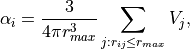
where  is the particle volume.
External heat flux
If add_external_heatflux is set to yes an external heat flux can be
imposed on particles directly, as described below.
Details on add_external_heatflux
The external application must be able to read the output created with the
output_settings command. This command will write
an empty file output_*_written.txt after it has completed its writing
indicating that the external application can start reading the VTK data.
The * indicates the time step that has just been written. It is
expected that the external application deletes this file once it has
completed its writing, otherwise a deadlock will occur. After this file deletion Aspherix will start
reading the external heat flux present in the particle data.
The heatFluxExternal field that is part of the particle data will be read after being written by an external program and will be imposed directly onto the particle.
In case add_external_heatflux_from_grid is set to yes an external heat
flux is distributed onto particles.
Details on add_external_heatflux_from_grid
This model works in combination with the calculate spatial_average command and allows using an external application to write a heat flux onto this Eulerian grid that is then distributed to all the particles in a cell of this grid.
See add_external_heatflux details above for how to write the data.
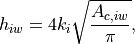
The additional heat flux a particle will see is thus

where  is the heat flux of the grid cell in which particle
is located and
is the heat flux of the grid cell in which particle
is located and  is the number of particles in this
grid cell.
is the number of particles in this
grid cell.
In case output_detailed_heatflux is set to yes additional per particle
properties are included in the output which contain the heat flux coming from
both conduction and radiation.
The heatFluxParticleConduction and heatFluxParticleRadiation
particle properties are created and output using the output_settings command which each contain the instanteaneous heat flux
a particle experiences due to conduction and radiation, respectively.
Coarse-graining information:
Using coarsegraining in combination with this command should lead to statistically equivalent dynamics and system state.
Output information
This command computes a scalar which can be accessed by various output
commands. This scalar is the total thermal energy of the particles in
the group associated with this command.
It can also be accessed using id_command-ID.total_thermal_energy.
The temperature, heat flux and heat source of an atom with index i can be obtained by
id_Temp[i], id_heatFlux[i] and id_heatSource[i], respectively.
This can be used to define variables, using the variable command, that can be
accessed by output commands.
Additional information
The particle temperature and heat source is written to binary restart files so simulations can continue properly.
Restrictions
Warning
The following functionalities do not have full GPU support: enable_radiation,
area_correction yes, modified_area_correction yes, store_contact_data yes
and dot access for the total thermal energy.