enable_electrical_conductivity command
Purpose
Enables calculation of DC current and heat generation by that current through the contact network
Syntax
enable_electrical_conductivity meshes meshList ...
mandatory keywords:
meshList = list of meshes to use
zero or more keyword/arg pairs may be appended
keyword = id or particle_group or enable_electric_heating or use_heat_conduction_area or skin_distance or verbose
id value = command-ID
  command-ID = user-assigned name for the command call
enable_electric_heating value = yes or no
  enables or disables heat generated by the electric currents
use_heat_conduction_area value = yes or no
  yes = corrected contact area used for heat conduction is also used to compute resistivity
  no = uncorrected contact area is used to compute resistivity
  For improved accuracy the default value is yes even when heat conduction is not enabled.
use_central_distance value = yes or no
  yes = use distance from centers to contact point as length of the "wire"
  no = use contact radius as "wire" length
solve_system value = yes or no
  yes = enable solving the electric equation system
  no = disable solving the electric equation system
skin_distance value = d_skin
  d_skin = distance a particle needs to travel to trigger solving the system
verbose value = yes or no
  yes = print information to screen and logfile
  no = do not print information to screen and logfile
Additionally, the behaviour of HYPRE, the library used to solve the underlying system of equations, can be controlled using the following keyword/arg pairs:
hypre_max_iterations value = nIter
  nIter = maximum number of iterations for the solver (default: 10000)
hypre_convergence_tolerance value = delta
  delta = convergence limit for matrix solver (default: 1e-7)
hypre_full_output value = yes or no
  yes = let hypre print convergence information to screen (requires verbose yes)
  no = don't print convergence information
Examples
# apply voltage boundary condition to two meshes
mesh id floor file meshes/floor.stl voltage 0.0
mesh id lid file meshes/lid.stl voltage 100.0
enable_electrical_conductivity id conductivity meshes {floor,lid}

# apply current boundary to lid and voltage boundary to floor
mesh id floor file meshes/floor.stl voltage 0.0
mesh id lid file meshes/lid.stl current 1e-5
enable_electrical_conductivity id conductivity meshes {floor,lid}
For meshes, access the calculated voltages and currents via:
id_floor.voltage
id_floor.current
id_lid.voltage
id_lid.current
Associated material properties
Material properties
specificElectricalResistance( ): specific resistance
of the material [
): specific resistance
of the material [ ]
]
Material interaction properties
contactResistancePrefactor( ): tunable prefactor
for contact resistance [-]
): tunable prefactor
for contact resistance [-]electricHeatingPrefactor( ): tunable prefactor for
heat generation [-]
): tunable prefactor for
heat generation [-]
Description
Consider particles confined by a geometry consisting of at least two
meshes. If these meshes are being held at certain
electrical voltage, or an electrical current is applied to at least one of the meshes,
a current will flow through the bed if there is
at least one continuous path from one mesh to the other along the
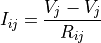
contact network. Each contact between particles  ,
,  can be assigned an electric resistance
(1)
where  is the contact area between the particles, is the
specific resistance,
is the contact area between the particles, is the
specific resistance,  is the length of the contact. In a similar
fashion, resistivities
is the length of the contact. In a similar
fashion, resistivities  can be computed for particles in contact
with a mesh. By default, the length of the contact is equal to the contact
radius:
can be computed for particles in contact
with a mesh. By default, the length of the contact is equal to the contact
radius: 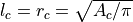 . If use_central_distance is set to
yes, the contact length is defined as
. If use_central_distance is set to
yes, the contact length is defined as
for particle-particle contacts with  ,
,  the
particle centers and
the
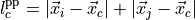
particle centers and  the contact point. For particle-wall
contacts, the contact length is given by
the contact point. For particle-wall
contacts, the contact length is given by
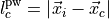
Furthermore, each particle has an electric potential (voltage)  ,
so from Ohm’s law, it directly follows that the current across a contact is
given by
,
so from Ohm’s law, it directly follows that the current across a contact is
given by
for a particle-particle contact and
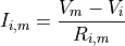
for a particle-mesh contact, where  is the electric
potential (voltage) of the mesh. The above equations can be written for each
particle-particle and particle-wall contact, and the resulting set of
equations can be recast into a matrix system
is the electric
potential (voltage) of the mesh. The above equations can be written for each
particle-particle and particle-wall contact, and the resulting set of
equations can be recast into a matrix system

where  is the matrix to be solved,
 is a vector whose elements represent the particle potentials and,
for meshes that use electrical current boundary conditions, the mesh potentials.
The vector
is a vector whose elements represent the particle potentials and,
for meshes that use electrical current boundary conditions, the mesh potentials.
The vector  has the values of the mesh potentials for particles
touching a mesh, zero values for particles without a mesh
contact, and the value of the mesh electrical current multiplied by the corresponding electrical resistance
for meshes that use the current boundary condition. The currents
has the values of the mesh potentials for particles
touching a mesh, zero values for particles without a mesh
contact, and the value of the mesh electrical current multiplied by the corresponding electrical resistance
for meshes that use the current boundary condition. The currents  across each contact are
computed from the connectivity and the potentials .
across each contact are
computed from the connectivity and the potentials .
Voltage or current boundary conditions can be specified by the keywords voltage and current,
respectively, of the meshe command.
If enabled, electric heat is generated following
(2)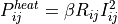
where is a tunable prefactor (see below).
The enable_electrical_conductivity command requires one parameter
in material_properties:
specificElectricalResistanceis the specific resistance of the material in Eq.1 in units of
 .
.
Additionally, two parameters are required in material_interaction_properties:
contactResistancePrefactoris the prefactor in
Eq.1. This parameter is dimensionless.electricHeatingPrefactoris the prefactor in
Eq.2. This parameter is dimensionless, and only needs to
be provided if enable_electric_heating yes.
The meshes keyword sets which meshes are being used: at least two meshes are needed. These meshes specify the boundary conditions of the conductivity problem, which are set by the voltage or current keywords of the meshes command.
If electrical potentials are used as boundary conditions, the corresponding values need to be different to cause any current to flow.
The meshes provided in the meshes list that do not specify any voltage or current use zero-valued current as the default boundary condition.
Setting enable_electric_heating to yes switches on heat generation by electric currents. The power generated at each contact is given by Eq.2
Note
if enable_electric_heating is activated, the user must also add the enable_heat_transfer command after enable_electrical_conductivity. The particle_group of enable_heat_transfer must be set to all.
If use_heat_conduction_area is enabled, the corrected contact area as defined in enable_heat_transfer is used to compute the resistances. This is useful if the Young’s Modulus is reduced to allow for lager simulation time steps. Please find more information on area correction in the documentation of the enable_heat_transfer command.
skin_distance controls the distance a particle needs to travel to trigger rebuilding and solving the system. Setting this to a low value will result in many solving steps. The system is also solved after every neighbor list build (see the neighbor_list command for details).
solve_system allows to set whether the system of equations is solved or not. This can be useful if setup steps (e.g. filling) need to be performed before solving for currents, since the enable_electrical_conductivity command must be defined before the first run or simulate command. Solving the equations can be enabled at any time using modify_command command (see below).
verbose yes prints additional information to screen and logfile after each iteration of the matrix solver.
The matrix system is solved using a conjugate gradient method. The behaviour of the solver can be configured using the following keywords:
hypre_max_iterations [value] sets the maximum number of iterations for the PCG solver. The default is 10000, which has been enough for systems up to 3 millions of particles. Increase if convergence was not reached at the end.
hypre_convergence_tolerance [value] controls when convergence is reached. If the residual differs by less than this value, convergence is assumed. The default is 1e-7.
hypre_full_output [yes/no] enables/disables printing of detailed information on convergence for each iteration.
Additional information
The voltage difference between two walls can be obtained using the calculate voltage command. The net electric current that passes through a wall can be calculated using the calculate electric_current command. The electric resistance of a compacted particle bed can be evaluated using the calculate electric_resistance command.
The electric potential can be accessed via id_[commandID]_potential where commandID is the id provided to this command via the id keyword. If heat conduction is enabled, the heat produced can be accessed via id_electricHeating. If these particle properties are available, output_settings will write them automatically. However, it is also possible to write these quantities explicitly by adding them to the particle_properties list of output_settings:
output_settings [....] particle_properties {id,id_conductivity_potential,id_heatSource}
Additionally, the conductance (inverse of the resistance) and absolute value of the current for each contact can be accessed by using calculate particle_contact_network and/or calculate wall_contact_network:
calculate particle_contact_network id pcn properties {pos,ids,electricConductance,electricCurrent}
calculate wall_contact_network id wcn properties {pos,ids,electricConductance,electricCurrent}
output_settings [ ... ] write_particle_contact_network yes particle_network_command_id pcn &
                        write_wall_contact_network yes wall_network_command_id wcn
Note
If the contact network commands are not defined and added by the user explicitly, some contact network information might not be present in the output file.
Computation of electric currents can be started and stopped via modify_command, for example
modify_command id conductivity old_style yes solve_system no
to halt computation and
modify_command id conductivity old_style yes solve_system yes
to resume. If electric heating is enabled, no heat will be generated for solve_system no.
For maximum performance, each multisphere or concave particle corresponds to a single node of the electric grid. Thus, if the individual atoms that form the multisphere/concave body are not in contact, electricity can still flow through the particle. The location of the electric node is given by the center of the bounding sphere of the multisphere/concave particle.
Restrictions
This command needs to appear before the first simulate or run command in the input script. There can only be one enable_electrical_conductivity command in the whole simulation. The values of the electrical potentials, currents and conductances are not restarted. This command is not available for particle shapes fiber and bonded. Due to the iterative nature of the system matrix solver, in some cases the current boundary conditions are satisfied only approximately, not exactly. However, the discrepancy is typically very small, and can be evaluated using the calculate electric_current command.
Warning
There are currently issues with periodic boundary conditions if both boundaries lie on the same processor. In this case, enable_electrical_conductivity might produce incorrect currents.
Default
group-ID = all, skin_distance = half of smallest radius in simulation, solve_system = yes,
enable_electric_heating = no, use_heat_conduction_area = yes, use_central_distance = no
Literature:
[1] Rickelt, Discrete Element Simulation and Experimental Validation of Conductive and Convective Heat Transfer in Moving Granular Material, PhD thesis (2011).