mesh_module wear
Purpose
Command for enabling wear of the mesh wall by particle impingement.
Syntax
mesh_module wear keyword value
Keywords:
Keywords |
Description |
|---|---|
id |
obligatory, user-defined name for the mesh module |
available models: finnie, finnie_unresolved, deformation, archard, combined, off |
|
specifies the output for total wear (
mass, volume)default:
volume |
Associated material properties
Material properties
hardness: material hardness used for the archard wear model [Pa]
Material interaction properties
k_finnie: coefficient for the finnie and finnie_unresolved wear models [m s2/kg]
k_deformation: coefficient for the deformation wear model [m s2/kg]
k_archard: coefficient for the archard wear model [-]
Examples
mesh_module wear id myWear model finnie
mesh_module wear id myWear model finnie_unresolved
mesh_module wear id myWear model archard
mesh_module wear id myWear model deformation
mesh_module wear id myWear model combined
After defining a mesh such as in
mesh id myMesh material steel file meshes/wall.stl mesh_modules { myWear }
The total eroded mass [Kg] and volume [m3] can be obtained via
id_myMesh.eroded_mass
id_myMesh.eroded_volume
With the combined model it is also possible to obtain the contribution of each individual wear mechanism to the total
wear mass:
id_myMesh.eroded_mass.archard
id_myMesh.eroded_mass.deformation
id_myMesh.eroded_mass.finnie_unresolved
and similarly for the eroded volume.
The local wear height [m], at each mesh element and at each output time step, is written to output files for further post processing e.g. in Paraview via
output_settings mesh_properties { wear }
The contribution of each wear mechanism to the total wear height will appear e.g. in the components tab of Paraview, together with the total wear.
Description
The mesh module wear is used to calculate the wear that a mesh experiences due to particle collisions. In order to reproduce different wear mechanisms, four wear models are available: archard, finnie, finnie_unresolved, deformation and combined wear. They reproduce the wear that results from sliding interactions, and the cutting and deformation produced in an impact. The models are described in detail below.
This mesh module is a prerequisite for the mesh module_deform.
Finnie Model
The model keyword with values finnie or finnie_unresolved activates two different modes of the
wear model developed by Finnie [1]. The former is based on the soft sphere framework and increments the wear at every
time step involved in a contact (see below), whereas the latter disconsiders the remaining contacts after the first impact i.e.
it is based on the hard sphere model.
This model for erosive
wear relates the rate of wear to the rate of kinetic energy of particle
impact on a surface. For finnie_unresolved, it reads
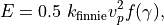
where  [m3/kg] is the worn volume (
 [m3]) resulting from a single particle colision
normalized by the particle mass (
[m3]) resulting from a single particle colision
normalized by the particle mass ( [kg]), i.e.
  ,
,  [m/s] is the magnitude of the particle impact velocity, [m s2/kg] is a model parameter and
  is a
dimensionless function of the impact angle between the approaching track and
the surface.
is a
dimensionless function of the impact angle between the approaching track and
the surface.
The model coefficient has to be specified as
in the following example:
material_properties steel density 8000 k_finnie 0.1 keywords values
where keyword/value denotes additional material properties (e.g., poissonsRatio,
coefficientRestitution, etc.).
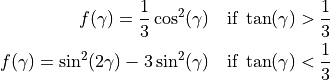
The function  is defined as
This model (finnie_unresolved) was formulated originaly in the framework of the hard sphere model. Here we also provide an alternative mode (finnie), adapted to the soft sphere model (see below).
When used
in conjunction with a Lagrangian particle tracks representing a constant mass flow rate of particles
of  , the eroded mass
  in kg during one time-step
 becomes
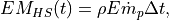
where  [kg/ m3] is the density of the worn material and the subscript HS denotes the hard sphere model. In contrast,
the soft sphere model resolves a particle-surface contact with multiple
time-steps, instead of one step, and therefore the corresponding formulation is adapted for that case.
[kg/ m3] is the density of the worn material and the subscript HS denotes the hard sphere model. In contrast,
the soft sphere model resolves a particle-surface contact with multiple
time-steps, instead of one step, and therefore the corresponding formulation is adapted for that case.
For model finnie the normalized worn volume is defined as
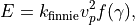
i.e. the definition of [m3/kg] is different than the finnie_unresolved by a factor of 0.5.
Considering a one term Taylor series expansion for the wear volume over small time intervals the variation
of the wear volume is obtained. A subsequent integration over one collision time leads to the following relation for
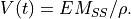
the eroded mass caused by one particle during the particle - surface contact:
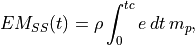
where  [s] is the contact time, the subscript SS denotes the soft sphere model, and
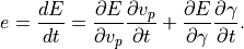
Since  is the dominant part of the time derivative and
tracking
is the dominant part of the time derivative and
tracking  would be computationally
tedious, the latter is neglected. Hence one obtains
would be computationally
tedious, the latter is neglected. Hence one obtains
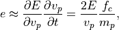
with  being the particle-surface contact force. Additionally,
 for
for  , where
  is the particle impact velocity vector, and
  is the surface normal vector (pointing into the surface) at the contact point. This follows from the assumption that
wear is caused only during the impact phase of the contact and not during
the repulsion phase. Thus,
is the surface normal vector (pointing into the surface) at the contact point. This follows from the assumption that
wear is caused only during the impact phase of the contact and not during
the repulsion phase. Thus,
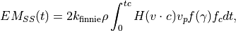
where  is the Heaviside function. For materials with a uniform density, the worn volume is easily obtained from the eroded mass:
The total worn volume in m3 and the total eroded mass in kg are simply the summation of  and
and  over
all mesh elements defining the solid object,
respectively. As mentioned earlier, the total worn volume or eroded mass are written in the output file
over
all mesh elements defining the solid object,
respectively. As mentioned earlier, the total worn volume or eroded mass are written in the output file simulation_data_aspherix.csv. The
sum_wear_output keyword with values volume or mass defines which option is output to this file. The default value is volume.
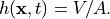
Since mass and volume are extensive thermodynamic properties, they can not be used to analyse the local wear at each point
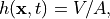
of the solid object. For a more refined, local analysis of the wear, we also provide the local wear height  [m], which is approximated by
the worn volume [m3] within the region demarcated by each mesh element normalized by the surface area of
the corresponding mesh element A [m2]:
[m], which is approximated by
the worn volume [m3] within the region demarcated by each mesh element normalized by the surface area of
the corresponding mesh element A [m2]:
The wear height [m] is output to the post folder and can be used to generate contour plots in Paraview for example.
In principle, the hard and soft sphere frameworks should give equivalent results when the Young’s modulus is made sufficiently large.
However, since the finnie and finnie_unresolved models use different definitions of [m3/kg], and therefore k_finnie, by a factor of 0.5,
the k_finnie would have to be adjusted by the same factor if the two models are compared in this limit condition.
Deformation Model
The impact deformation wear model is similar to the finnie_unresolved model but the corresponding equation is
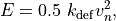
where  [m/s] is the velocity component normal to the wall at the impact point.
Other variables have the same meaning as in the impact cutting model. The value of the model coefficient
[m s2/kg] is set by the material property
[m/s] is the velocity component normal to the wall at the impact point.
Other variables have the same meaning as in the impact cutting model. The value of the model coefficient
[m s2/kg] is set by the material property k_deformation.
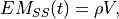
Archard Model
The model keyword with value archard activates the model proposed by Archard
[2]. The model calculates the total worn volume [m3]
according to the following equation:
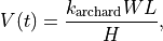
where is a non-dimensional constant,  [N] is the total normal load,
  [m] is
the sliding distance (integrated tangential velocity) and [Pa] the
hardness of the softest contact surface. The model coefficient
[m] is
the sliding distance (integrated tangential velocity) and [Pa] the
hardness of the softest contact surface. The model coefficient  and
the hardness have to be specified for each material pair and each
material, respectively. A corresponding section in the input script could look
like below:
and
the hardness have to be specified for each material pair and each
material, respectively. A corresponding section in the input script could look
like below:
material_properties steel density 8000 k_archard 1.0 hardness 2000.0 keywords values
material_properties plastic density 1200 k_archard 0.9 hardness 1000.0 keywords values
material_interaction_properties plastic steel k_archard 0.9 keywords values
where keywords/values denote additional material properties (e.g., poissonsRatio,
coefficientRestitution, etc.).
The eroded mass and local wear height are easily obtained from the worn volume:
and
respectively.
Combined Model
The model keyword with value combined activates the combined wear model developed by Roessler and Katterfeld [3].
In this case, the total wear is the result of the sum of the wear obtained from three different wear mechanism: impact cutting (finnie_unresolved),
impact deformation (deformation), and sliding (archard). This model is able to predict the wear in a variety of different conditions,
and it is shown by Roessler and Katterfeld to be the most robust combination of different models. The equation for the
worn volume per unit of particle mass is
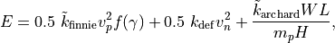
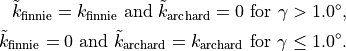
where the coefficients  and
and  are given by
Additional information
This mesh module stores a global scalar for access by various output
commands. The output value is accessed via the
property name, which is wear, e.g. id_myMesh.wear. This scalar contains the
local wear height at each mesh element.
Alternatively for backward compatibility the access via data position in square
brackets is also possible. The position of the data in the output depends on
the additional mesh modules that are used (in case of mesh/surface/stress/6dof
there are 9 components for mesh/surface/stress, the output for the wear module
comes afterwards). Therefore, for a mesh with id myMesh, the wear value can be
accessed via id_myMesh[10].
See the table below for an overview of the available properties and how to access them.
Mesh module property |
property name (dot access) |
probable array position |
wear volume or mass |
wear |
10 |
eroded volume |
eroded_volume |
11 |
eroded mass |
eroded_mass |
12 |
For the combined wear model the contributions of each wear mechanism are also added to this vector.
Be aware that using the keyword calculate sum with mesh_properties {wear} will calculate the sum of [m]
(and not or ) over all mesh elements defining the solid object. By definition of , this summation
grows without bounds in the limit of mesh refinement and therefore its use is not recommended. If one wishes to analyse
the total worn volume or eroded mass, one can find these quantities in the simulation_data_aspherix.csv file, as explained earlier.
Alternatively, it is also possible to define a variable storing or and output its values to a user defined file,
which is illustrated below for .
calculate sum id totalWearVolume meshes {mesh_user} mesh_properties {wear} property_weights {area}
write_to_file string 'id_time id_totalWearVolume[1]' file post/wear_data.txt title 'time total_wear_volume'
Details about the usage of the modify command
Using the modify_command, the wear can be reset via the
wear/reset_wear option (old_style must be set to ‘yes’).
References
[1] Finnie, Iain. Erosion of surfaces by solid particles. Wear 3.2 (1960): 87-103.
[2] Archard, JeFoa. Contact and rubbing of flat surfaces. Journal of applied physics (1953): 24(8), 981-988.
[3] Roessler, T. and Katterfeld, A. Calibrated and Validated Wear Prediction for Bulk Material Handling Equipment using DEM Simulations. ICBMH2023 - The 14th International Conference on Bulk Materials Storage, Handling and Transportation 11-13th July, 2023, Wollongong, New South Wales, Australia.