Postprocessing & data visualization
Description:
This is a collection of different hints for postprocessing.
Introduction:
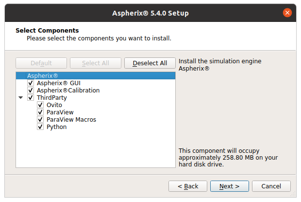
Two tools are recommended for graphical postprocessing of Aspherix® simulation results - Paraview (https://www.paraview.org/) and Ovito (https://www.ovito.org/). Both tools are distributed with the installer and can be installed as third party components.
Together with the Ovito and Paraview the installer contains a set of “Paraview Macros” that can be used for automated postprocessing. These macros extract particles, meshes, the simulation domain, particle-particle and particle-wall contact data and Eulerian field data (if they exist). Ovito automatically loads all data sets separately when opening the aspherix_simulation.pvd file (auto-generated in the post folder when using the output_settings command and default folder).
In the following two sections we will briefly show how to postprocess in Paraview and in Ovito.
For more detailed information about the capabilities please check the documentation of the respective software package:
Paraview: https://docs.paraview.org/en/latest/ Ovito: https://docs.ovito.org/
Postprocessing with Paraview
For using the provided macros to postprocess simulation data with Paraview it is strongly recommended to install the Paraview version that is distributed with Aspherix. For a successful usage of the macro at least Paraview 5.8.0 or newer is required.
For applying the macro please launch Paraview and load the aspherix_simulation.pvd file that is automatically generated by the output_settings command and that can be found in the post folder of the simulation. This file contains all information about the generated simulation output.
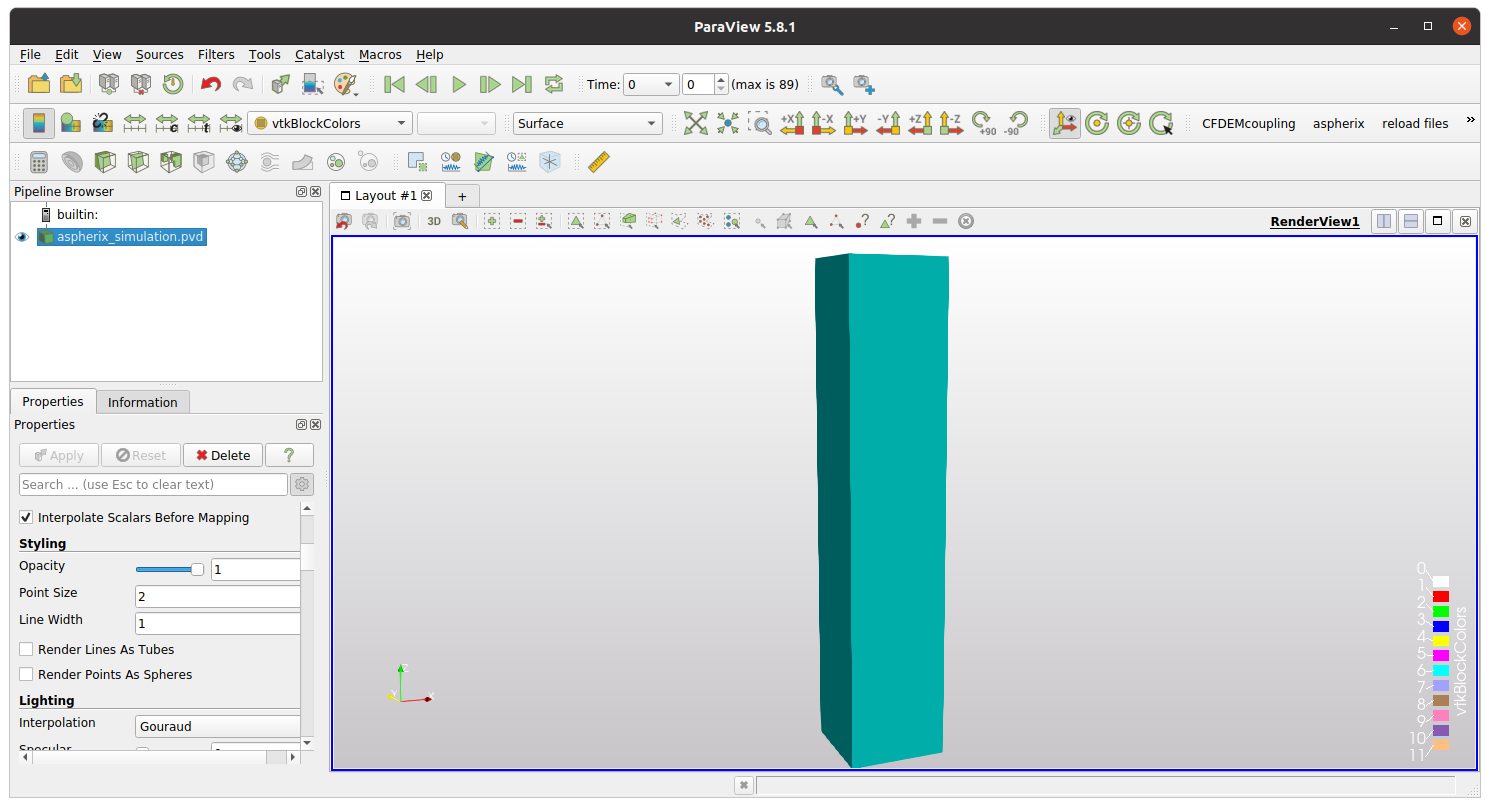
Make sure that the item is selected in the Pipline browser and click on the aspherix button that is shown.
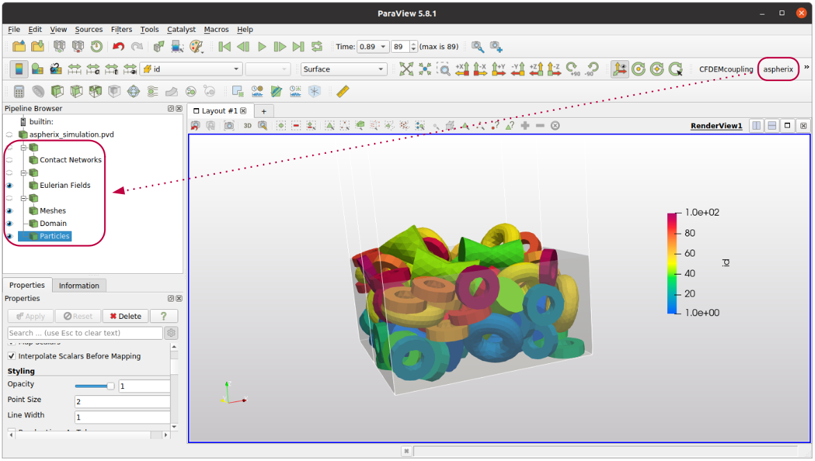
This automatically extracts the data blocks that contain meshes, particles, contact networks (if there are any), Eulerian grid data (if there is any) and the decomposed simulation domain. All filters that are used can also be found in Filters/Alphabetical/Aspherix FILTERNAME.
Note
By default the macros are installed to $HOME/.config/ParaView/Macros or $HOME/AppData/Roaming/ParaView/Macros on Linux and Windows, respectively. As a backup they are also located in your Aspherix installation path under share/ParaView.
Basic Postprocessing in Paraview with Macro
This brief getting-started section on postprocessing is based on the output of the chute wear example (examples/solver/basic/chute_wear).
Please open Paraview and open the file aspherix_simulation.pvd which was written to the post_n folder. Then apply the aspherix macro as described above. The simulation data is automatically visualized:
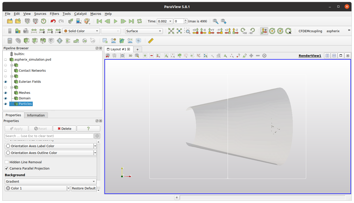
It becomes visible that the current simulation contains data files for 500 time steps (from 0 to 499). One can use the buttons or the text field to navigate to an arbitrary time step. By pressing the play button the simulation results are animated.

Per default the particles are colored with “solid color”. For changing to a quantity from the simulation please select the Particles object in the Pipeline Browser and toggle the properties selector to the desired quantity (e.g., v for velocity):
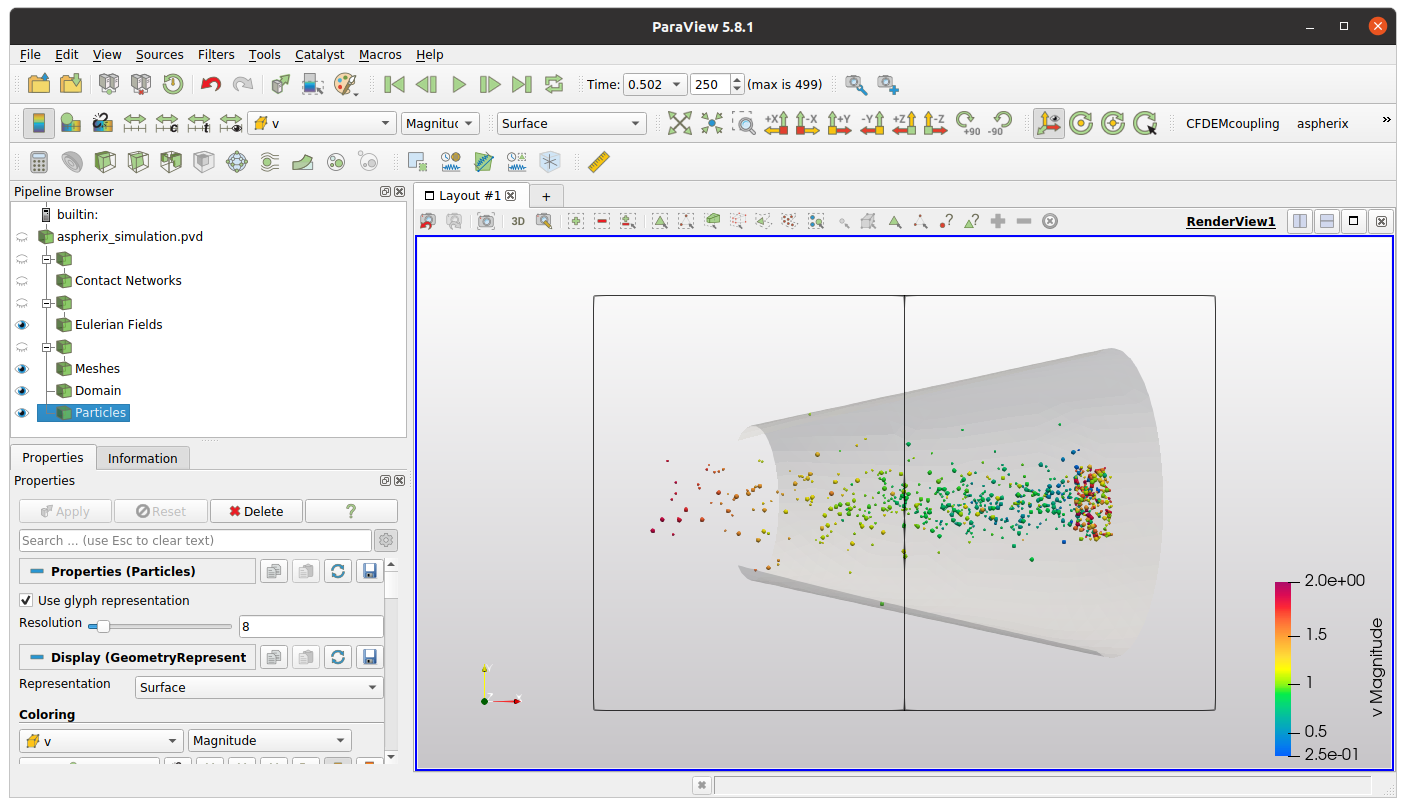
For a better visibility we have also changed the solid color of the domain from white to black (in the Properties Window / Coloring, Edit button).
Also the meshes can be colored according to calculated quantities such as the wear in this case:
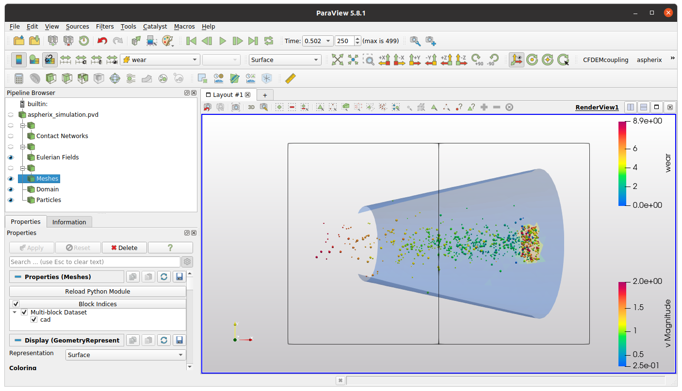
Per default all meshes are displayed with an opacity of 0.3. This can be changed in the Properties Window (below Pipeline Browser) / Styling / Opacity.
When running simulations with bonded particles, or when particle-particle contacts are added to the output (output_settings command, write_particle_contact_network / write_wall_contact_network) the contact networks are extracted by the Paraview macro and can be visualized:
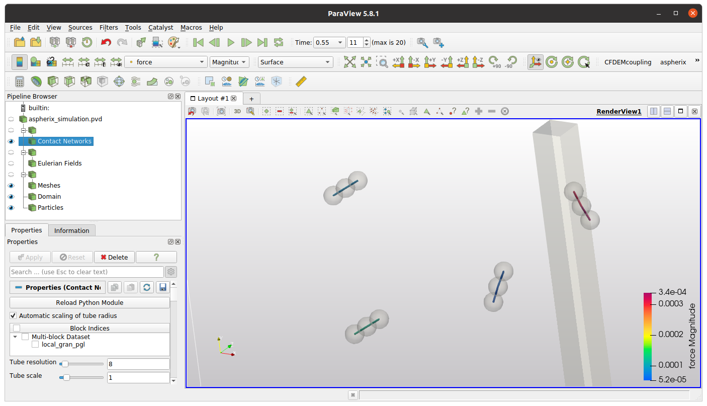
This image is based on the test case (examples/solver/contact_models/bonded_particles), the particles have solid color and an opacity value of 0.3.
When simulations write Eulerian data (e.g., due to a calculate spatial_average command) the information is automatically extracted by the ParaView macros:
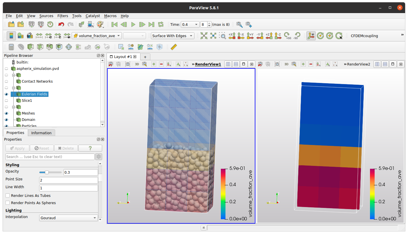
This image is based on a test case (examples/solver/postprocessing/spatial_averaging), the Eulerian Field in colored according to the average volume fraction in the cells. The view is split, on the right hand we show a slice filter, applied to the Eulerian data.
Basic Postprocessing in Ovito
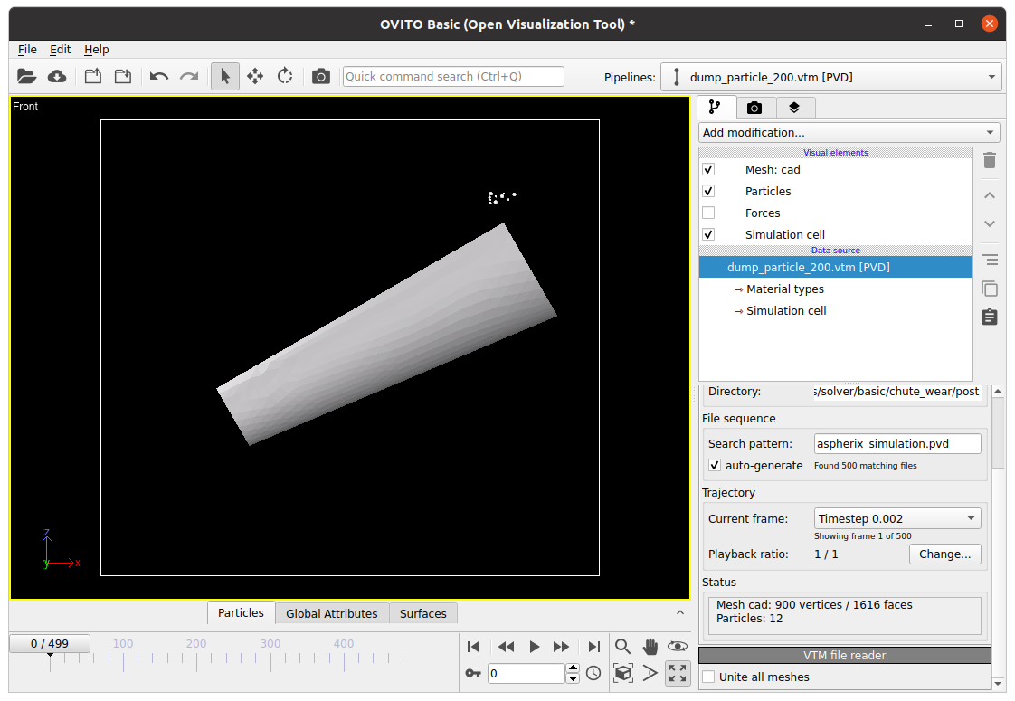
When opening the aspherix_simulation.pvd file, Ovito automatically extracts the different visual elements (in this case one mesh, particles, forces and simulation cell):
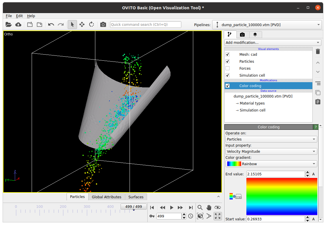
For coloring particles, we click on “Add modification” (above list of visual elements”) and select “Color coding” from the list. Please make sure that “Particles” is selected in “Operate on”. In this case, Ovito colors the particles according to the velocity magnitude automatically:
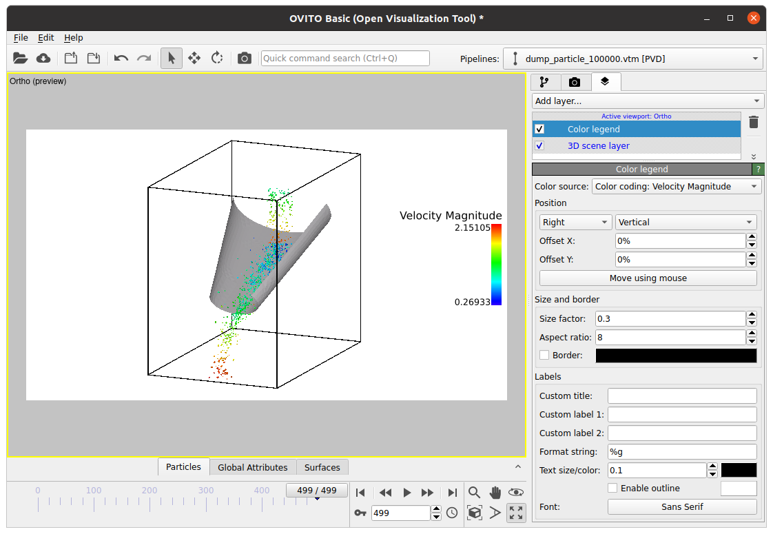
If necessary, adjust the range of the color bar. To add a legend to the visual area, please toggle to the layer view and add a layer of type “Color legend”:
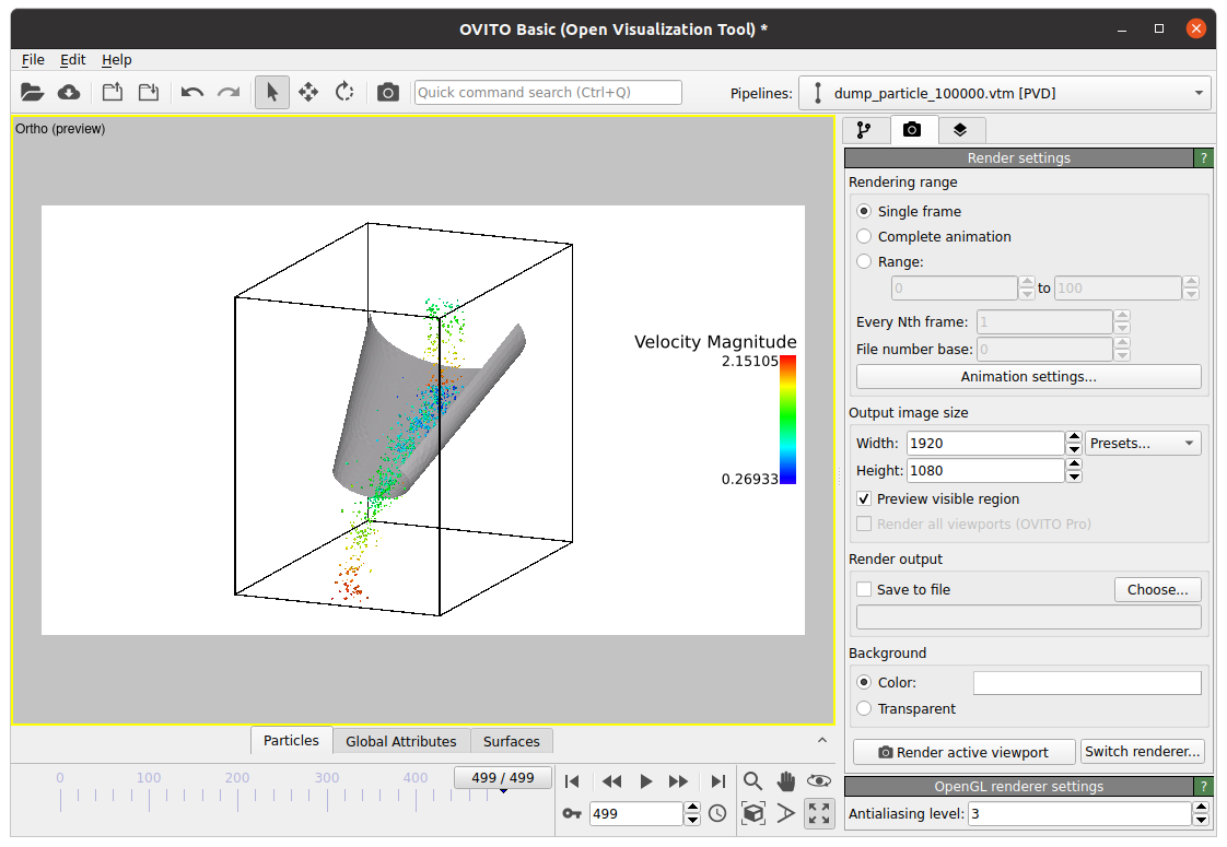
For obtaining this view, the “Preview visible region” checkmark must be set in the Render settings tab:
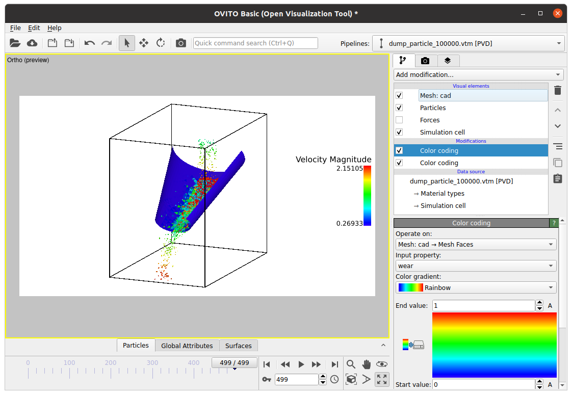
Also for mesh coloring we add a modification. This time we let the color coding operate on “Mesh: cad -> Mesh Faces” and chose wear as input property:
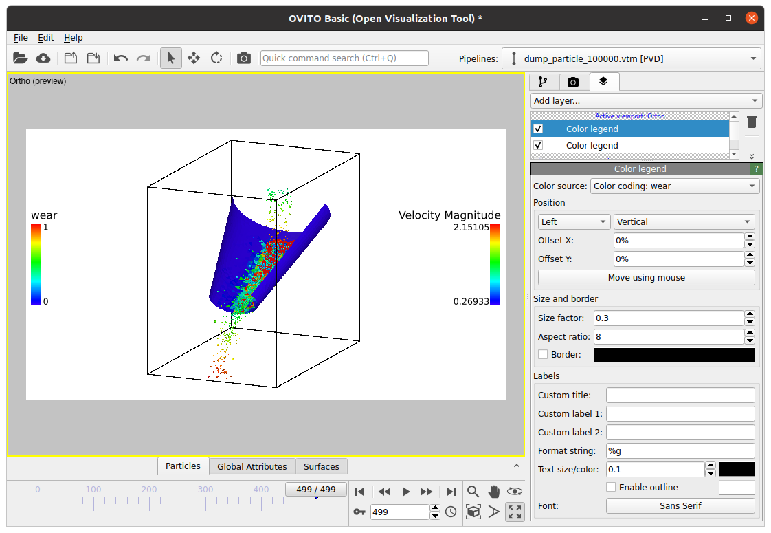
For obtaining a second legend, we add another color legend layer:
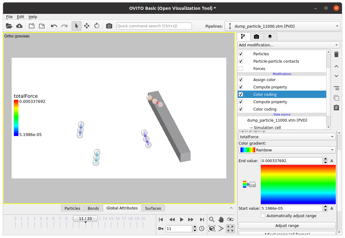
When a particle-particle contact network is available in the result files, Ovito automatically loads the “Particle-particle contacts”. To obtain the following image we
applied a “Compute property” filter to the particles; The output property was set to “Transparency” (please type to text field), the expression was set to 0.3.
ticked the check mark for “Particle-particle contacts”.
set the bond width to 0.002 in the Bonds display window.
calculated the total force of the bonds with a compute property. Output property: totalForce; Expression: sqrt(force.1*force.1+force.2*force.2+force.3*force.3)
used a Color coding modification for the bonds, Input property: totalForce
added a “Color layer” of type “Color legend”.
Note: the visualization of particle-wall contacts and particle-particle contacts in periodic cases is currently not available in Ovito.
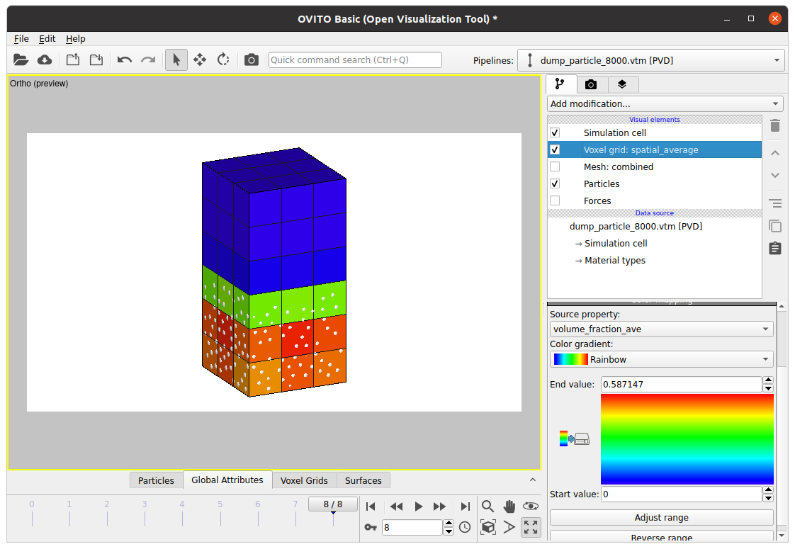
If simulation output contains eulerian grid data, it is automatically extracted when the results are loaded. For visualizing the data, please just tick the check box next to “Voxel grid: spatial_average”. Then you can select any of the available source properties in the color mapping section (e.g., volume_fraction_ave):
Note
Please note that Ovito offers the choice between loading all meshes separately and loading them as a combined component. For the latter please select the data set in the Data source area and set the check mark for “Unite all meshes” in the VTM file reader.
The Ovito version that comes with Aspherix is Ovito Basic. There is also Ovito Pro which offers additional features such as high-quality image and movie generation, powerful data analysis tools, a Python-based scripting interface and professional software support. Should you be intrigued, head over to Ovito.org <https://www.ovito.org/about/ovito-pro/> to discover more.
Questions?
For more detailed information about the capabilities please check the documentation of the respective software package:
Paraview: https://docs.paraview.org/en/latest/ Ovito: https://docs.ovito.org/
If any questions remain, contact us.