define_lattice command
Purpose
Command to define global grid for structured particle creation.
Note
This command is supported by Aspherix GPU.Syntax
define_lattice keyword value
Keywords |
Description |
|---|---|
obligatory; available options: |
|
lattice spacing in distance units (reduced density
rho* in LJ units)units: [length]
|
|
vector of fractions of a unit cell (0 <= x,y,z < 1)
default: (0,0,0)
|
|
dimension (
x, y or z) and vector of integer lattice directionsdefault: x (1,0,0), y (0,1,0), z (0,0,1)
|
|
vector of lattice spacings in the x,y,z box directions
units: [length]
|
|
available for mode
customprimitive vector that defines unit cell
default: a1 = (1,0,0), a2 = (0,1,0), a3 = (0,0,1)
|
|
available for mode
customfractional vector of a basis particle (0 <= x,y,z < 1)
|
Examples
define_lattice mode sq scale 0.1
define_lattice mode bcc scale 0.1 origin (0.5, 0, 0) orient x (1, 2, 1)
define_lattice mode custom scale 0.1 a1 (1, 0, 0) a2 (0.5, 1, 0) a3 (0, 0, 0.5) &
                                     basis (0, 0, 0) basis (0.5, 0.5, 0.5)
Description
Define a lattice for use by other commands. A lattice is simply a set of points in space, determined by a unit cell with basis particles, that is replicated infinitely in all dimensions. The arguments of the lattice command can be used to define a wide variety of crystallographic lattices.
A lattice is used in two ways. First, the create_particles command creates particles on the lattice points inside the simulation box. Note that the create_particles command allows different materials to be assigned to different basis particles of the lattice. Second, the lattice spacing in the x,y,z dimensions implied by the lattice, can be used by other commands as distance units (e.g. create_box, region and velocity), which are often convenient to use when the underlying problem geometry is particles on a lattice.
The lattice mode must be consistent with the dimension of the
simulation - see the dimension command. Modes sc
or bcc or fcc or hcp or diamond are for 3d problems. Modes
sq or sq2 or hex are for 2d problems. Mode custom can be
used for either 2d or 3d problems.
A lattice consists of a unit cell, a set of basis particles within that
cell, and a set of transformation parameters (scale, origin,`` orient``)
that map the unit cell into the simulation box. The vectors a1,a2,a3
are the edge vectors of the unit cell. This is the nomenclature for
“primitive” vectors in solid-state crystallography, but the
unit cell they determine does not have to be a “primitive cell” of
minimum volume.
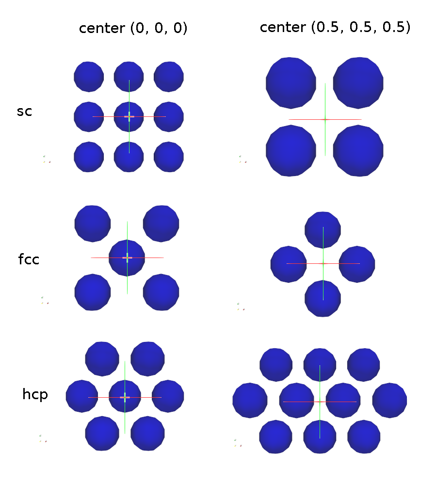
This image shows examples for the sc, the fcc and the hcp pattern, once with the center equal to the origin, and once replaced by 0.5 in each direction. Please note that the examples show the patterns in 2D for better visibility:
A lattice of mode none does not define a unit cell and basis set,
so it cannot be used with the create_particles
command. However it does define a lattice spacing via the specified
scale parameter. As explained above the lattice spacings in x,y,z can
be used by other commands as distance units. No additional
keyword/value pairs can be specified for the none mode. By
default, a define_lattice mode none scale 1.0 is defined, which means
the lattice spacing is the same as one distance unit, as defined by the
units command.
Lattices of mode sc, fcc, bcc, and diamond are 3d lattices that define
a cubic unit cell with edge length = 1.0. This means a1 = (1, 0, 0), a2 = (0,
1, 0), and a3 = (0, 0, 1). Mode hcp has a1 = (1, 0, 0), a2 = (0, ,sqrt(3), 0),
and a3 = (0, 0, sqrt(8/3)). The placement of the basis particles within the
unit cell are described in any solid-state physics text. A sc lattice has 1
basis particle at the lower-left-bottom corner of the cube. A bcc lattice
has 2 basis particles, one at the corner and one at the center of the cube. A
fcc lattice has 4 basis particles, one at the corner and 3 at the cube face
centers. A hcp lattice has 4 basis particles, two in the z = 0 plane and 2
in the z = 0.5 plane. A diamond lattice has 8 basis particles.
Lattices of mode sq and sq2 are 2d lattices that define a square unit cell
with edge length = 1.0. This means a1 = (1, 0, 0) and a2 = (0, 1, 0). A sq
lattice has 1 basis particle at the lower-left corner of the square. A sq2
lattice has 2 basis particles, one at the corner and one at the center of the
square. A hex mode is also a 2d lattice, but the unit cell is rectangular,
with a1 = (1, 0, 0) and a2 = (0, sqrt(3), 0) It has 2 basis particles, one at
the corner and one at the center of the rectangle.
A lattice of mode custom allows you to specify a1, a2, a3, and a
list of basis particles to put in the unit cell. By default, a1 and a2
and a3 are 3 orthogonal unit vectors (edges of a unit cube). But you
can specify them to be of any length and non-orthogonal to each other,
so that they describe a tilted parallelepiped. Via the basis
keyword you add particles, one at a time, to the unit cell. Its arguments
are fractional coordinates (0.0 <= x,y,z < 1.0), so that a value of
0.5 means a position half-way across the unit cell in that dimension.
This sub-section discusses the arguments that determine how the idealized unit cell is transformed into a lattice of points within the simulation box.
The scale argument determines how the size of the unit cell will be
scaled when mapping it into the simulation box. I.e. it determines a
multiplicative factor to apply to the unit cell, to convert it to a
lattice of the desired size and distance units in the simulation box.
The meaning of the scale argument depends on the units
being used in your simulation.
For all unit styles except lj, the scale argument is specified in
the distance units defined by the unit style. For example, in real
or metal units, if the unit cell is a unit cube with edge length
1.0, specifying scale = 3.52 would create a cubic lattice with a
spacing of 3.52 Angstroms. In cgs units, the spacing would be 3.52
cm.
For unit style lj, the scale argument is the Lennard-Jones reduced density,
typically written as  . Aspherix® converts this value into the
multiplicative factor via the formula
. Aspherix® converts this value into the
multiplicative factor via the formula 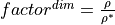 ,
where
,
where  with V = the volume of the
lattice unit cell and N = the number of basis particles in the unit cell
(described below), and dim = 2 or 3 for the dimensionality of the simulation.
Effectively, this means that if LJ particles of size sigma = 1.0 are used in
the simulation, the lattice of particles will be at the desired reduced
density.
with V = the volume of the
lattice unit cell and N = the number of basis particles in the unit cell
(described below), and dim = 2 or 3 for the dimensionality of the simulation.
Effectively, this means that if LJ particles of size sigma = 1.0 are used in
the simulation, the lattice of particles will be at the desired reduced
density.
The origin option specifies how the unit cell will be shifted or
translated when mapping it into the simulation box. The x,y,z values
are fractional values (0.0 <= x,y,z < 1.0) meaning shift the lattice
by a fraction of the lattice spacing in each dimension. The meaning
of “lattice spacing” is discussed below.
The orient option specifies how the unit cell will be rotated when
mapping it into the simulation box. The dim argument is one of the
3 coordinate axes in the simulation box. The other 3 arguments are
the crystallographic direction in the lattice that you want to orient
along that axis, specified as integers. E.g. “orient x (2, 1, 0)” means
the x-axis in the simulation box will be the [210] lattice
direction. The 3 lattice directions you specify must be mutually
orthogonal and obey the right-hand rule, i.e. (X cross Y) points in
the Z direction. Note that this description is really only valid for
orthogonal lattices. If you are using the more general lattice mode
custom with non-orthogonal a1,a2,a3 vectors, then think of the 3
orient options as creating a 3x3 rotation matrix which is applied to
a1,a2,a3 to rotate the original unit cell to a new orientation in the
simulation box.
Several commands have the option to use distance units that are inferred from “lattice spacing” in the x,y,z box directions. E.g. the region command can create a block of size 10x20x20, where 10 means 10 lattice spacings in the x direction.
The spacing option sets the 3 lattice spacings directly. All must
be non-zero (use 1.0 for dz in a 2d simulation). The specified values
are multiplied by the multiplicative factor described above that is
associated with the scale factor. Thus a spacing of 1.0 means one
unit cell independent of the scale factor. This option can be useful
if the computed spacings are inconvenient to use in subsequent
commands, which can be the case for non-orthogonal or rotated
lattices.
If the spacing option is not specified, the lattice spacings are
computed in the following way. A unit cell of the lattice
is mapped into the simulation box (scaled, shifted, rotated), so that
it now has (perhaps) a modified size and orientation. The lattice
spacing in X is defined as the difference between the min/max extent
of the x coordinates of the 8 corner points of the modified unit cell.
Similarly, the Y and Z lattice spacings are defined as the difference
in the min/max of the y and z coordinates.
Note that if the unit cell is orthogonal with axis-aligned edges (not
rotated via the orient keyword), then the lattice spacings in each
dimension are simply the scale factor (described above) multiplied by
the length of a1,a2,a3. Thus a hex mode lattice with a scale
factor of 3.0 Angstroms, would have a lattice spacing of 3.0 in x and
3*sqrt(3.0) in y.
Warning
For non-orthogonal unit cells and/or when a rotation
is applied via the orient keyword, then the lattice spacings may be
less intuitive. In particular, in these cases, there is no guarantee
that the lattice spacing is an integer multiple of the periodicity of
the lattice in that direction. Thus, if you create an orthogonal
periodic simulation box whose size in a dimension is a multiple of the
lattice spacing, and then fill it with particles via the
create_particles command, you will NOT necessarily
create a periodic system. I.e. particles may overlap incorrectly at the
faces of the simulation box.
Regardless of these issues, the values of the lattice spacings calculated are printed out, so their effect in commands that use the spacings should be decipherable.
Additional information
No information about this command is written to binary restart files.
Restrictions
The
a1,a2,a3,basiskeywords can only be used with modecustom.